Bivariate Cross-trait Genetic Architecture Analyses of GWAS

Welcome to the 1.1.2 version of our website. Despite being in the early stages of development, our platform is equipped with a diverse range of tools and methods for genetic and epidemiological analysis. We recognize the dynamic and continuous development in these fields. Therefore, our team is committed to updating and expanding our platform to incorporate more advanced and useful tools. We are always interested in hearing back from you. If you have recommendations for additional tools or methods that could enrich our platform, please feel free to share them with us. Your insights and expertise will undoubtedly contribute to the development of our platform and benefit other users worldwide. This is an ongoing project for us, so stay tuned for more exciting updates and advancements in the future. We appreciate your patience and your support as we work diligently to implement more methods and improve your experience on our site.

BIGA GWAS Team

Documentation of BIGA GWAS

Version:

This guide is created as a reference for navigating our platform's diverse features with ease. In this manual, you will find an outline of the data specifications needed to get started, a walkthrough of the platform's backend configurations, and an explanation of all the functionalities.

1. Data Processing

1.1 Data Processing Diagram
1.2 Summary Statistics File Format and Content requirements
1.3 Build Input Files
1.4 Data Harmonization Pipeline
1.5 Harmonization Codes
1.6 Query Data from GWAS Catalog
1.7 Query Data from IEU OpenGWAS
1.8 Query Data from Neale Lab

2. Curated Datasets

2.1 Brain and Organ Imaging Traits
2.2 UK Biobank (Neale Lab)
2.3 UKB Oxford Brain Imaging Traits
2.4 Biobank Japan
2.5 UKB-PPP European Protein GWAS
2.6 FinnGen
2.7 PGC (Psychiatric Genomics Consortium) and Other Brain Disorders
2.8 GWAS Catalog
2.9 CHIMGEN

3. Analysis

3.1 Massive LDSC Analysis
3.2 Massive SumHer Analysis
3.3 Massive LAVA Analysis
3.4 Massive POPCORN Analysis
3.5 Pairwise Analysis

4. Analysis Results and Log Files

4.1 Analysis Results
4.2 BIGA Log Files

5. Queue System and Periodic Jobs

5.1 Queue System
5.2 Periodic Jobs

6. Other Functions

6.1 Email Notification
6.2 Public Data
6.3 Public Results

7. Description examples

7.1 Method: LDSC
7.2 Method: SumHer
7.3 Method: LAVA
7.4 Method: Popcorn

1. Data Processing

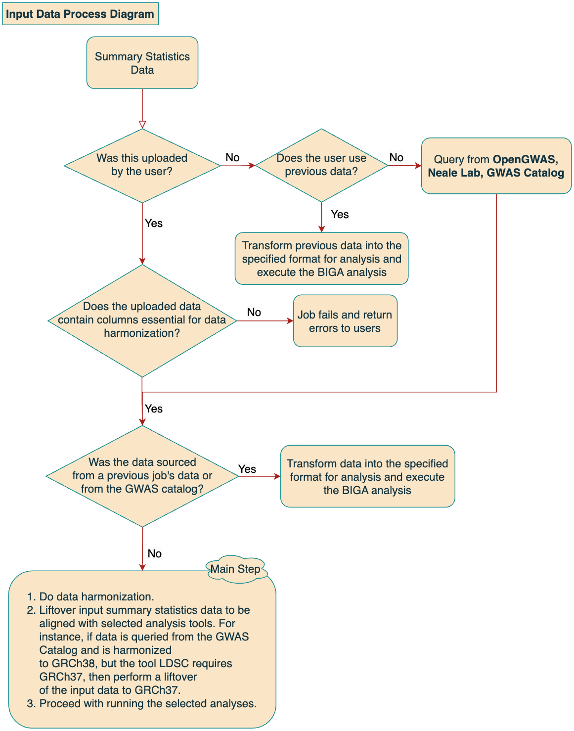
1.1 Data Processing Diagram

This diagram illustrates how BIGA process user-input files.

1.2 Table 1. Required columns for harmonization and BIGA analysis

The table gives the column requirements for users' uploaded input files. It is also the standard format on BIGA, which is able to perform LDSC, LAVA, Popcorn, SumHer analyses.

Index	Column Name	Description	Type
1	chr	Indicates the chromosome where the single nucleotide polymorphism (SNP) is located	Require either chr,position or snp column.
2	position	Refers to the specific base pair position of the SNP on the chromosome
3	snp	Identifier for the SNP (e.g.,rsID)
4	a1	Effect allele (allele associated with the risk of disease)	Mandatory
5	a2	Other allele (non-effect allele)	Mandatory
6	beta	Refers to the estimated effect size of a particular genetic variant on a trait or disease. (beta > 0 means that effect allele (a1) increases disease risk).	Require either beta or odds_ratio column
6	odds_ratio	Odds ratio (1 indicates no effect; above 1 indicates effect allele (a1) increases disease risk)	Require either beta or odds_ratio column
7	se	Standard error, a smaller standard error indicates a more reliable estimate of the beta/odds_ratio coefficient	Mandatory
8	eaf	Effect allele frequency, the frequency of the effect allele (a1) in the study population	Mandatory
9	pvalue	Indicates the statistical significance of the association between the SNP and the trait being studied	Mandatory
10	n	Sample size, the number of individuals or samples included in the study	Mandatory
11	z	Z-score (0 means no association between a genetic variant and disease risk; above than 0 indicates an increased risk associated with the variant)	Optional

1.3 Build Input Files

For both the Massive Analysis and Pairwise Analysis processes in BIGA, user can input their GWAS summary statistics. BIGA transforms input files into a standard format (harmonized and compatible to all analysis methods). You have three options for providing the input data:

1. Upload data
2. Use the Query data function
3. Use previous data

For the Upload data option, BIGA accepts files in .txt and .gz formats. For a gzipped file, please include only one plain text file. The uploaded file size should not exceed 600 Mb. The uploaded file can either be space-separated or tab-separated. Due to this format, please ensure that each element, including column names, does not contain any spaces. Additionally, make sure your data does not have repeated column names. Your input GWAS summary statistics should meet the column requirements, detailed in Table 1, to ensure proper data harmonization and further analysis. The headers of your uploaded file will be compared with the column requirements before harmonization. If the headers don't match our requirements, the job will be rejected. It is not necessary for the column names to be identical with the column names in Table 1. BIGA automatically identifies columns using similar to those used by the LDSC munge file. However, we recommend manually specifying as many column names as possible to prevent incorrect column matching.

Header Detection Rules

Missing value

Missing value can be written as "." or "NA" in the input file.

Parameters

Specify the Human Genome Build version (GRCh37 or GRCh38) if your data does not include a snp column for rsID and instead includes chromosome and position columns.
For data built on GRCh37, BIGA will convert it to GRCh38 using the liftOver Python package with the chainfile provided by UCSC (https://hgdownload.cse.ucsc.edu/goldenpath/hg19/liftOver/, hg19ToHg38.over.chain.gz). Rows that cannot be aligned to a new position in GRCh38 will be removed.
For data built on GRCh38, BIGA will skip chromosome and position alignment process with the reference chainfile.
The trait name of your uploaded file should be specified, please ensure your trait name does not include any spaces.
The population (European or East Asian) of your uploaded file should be specified.

Notes

BIGA assumes that the position field in the uploaded file uses a 1-based coordinate system. Rows containing chromosome X, Y, or M will also be excluded from the process. The pipeline currently supports human genome version GRCh37 and GRCh38. If your data is created based on an older version of the human genome e.g. NCBI36, you will need to update the genomic positions using the liftOver tool from UCSC. However, if your data includes snp column, position update is not required. BIGA will automatically update the chromosome and position information to align with the latest dbSNP build 156 version. In analyses like LDSC, LAVA, POPCORN, and SumHer, the effect_allele and other_allele columns are interpreted as A1 and A2, respectively. If both odds_ratio and beta are present, LDSC uses beta as the signed summary statistics.

For Query data option, BIGA can directly query data from three external data resources:

1. GWAS Catalog
2. IEU OpenGWAS
3. Neale Lab

GWAS Catalog Data

BIGA supports querying of data from the GWAS Catalog, where the data should be FTP accessible and should already be harmonized by GWAS Catalog platform. BIGA provides a daily-updated GWAS Catalog harmonized list (Table 2). Since the data has been harmonized, BIGA will skip the harmonization step. You are required to input only the trait ID and sample size, after which BIGA will manage the FTP download. Once downloaded, BIGA converts the data into its universal format, incorporating columns snp, chr, position, pvalue, eaf, a1, a2, n, odds_ratio or beta, and se. The harmonized file from the GWAS Catalog might present diverse column names to represent harmonized columns. For instance, beta could be labeled as hm_beta or beta. BIGA first checks for hm_beta; if absent, it defaults to the beta column. Queries will be rejected if the proportion of missing values in any harmonized column exceeds 50% or if essential fields are missing.

IEU OpenGWAS Data

BIGA supports querying of data from IEU OpenGWAS, where the data should be downloadable via the OpenGWAS website. You need to input the trait ID and the sample size, which can be found in OpenGWAS. The download files include a summary statistics VCF file and its corresponding index file. BIGA then transforms the original VCF files into its universal format, interpreting ID as snp, CHROM as chr, POS as position, LP as negative log p-value, AF1 as eaf, ALT as a1, REF as a2, ES as beta (If the trait is binary, logOR will be interpreted as beta), and SE as se. Given that IEU OpenGWAS data might not be harmonized, BIGA performs the harmonization step for any data acquired from this source. Since the original file includes a snp column, specifying the human genome build version is unnecessary. Additionally, data missing the required columns or with more than 80% missing values will not be successfully queried.
Note: If a user queries the trait from IEU OpenGWAS, the harmonized data will be stored on our cloud server. Should another user select this data, BIGA will use it directly instead of re-querying it.

Neale Lab Data

Data from Neale Lab has been pre-downloaded and harmonized by BIGA for your convenience. You can find a comprehensive list of available traits in Table 3, which includes both Trait IDs and Phenotype descriptions. To facilitate your search for a specific trait or disease, you can simply enter a trait, such as bmi, into the search field. This action will display all traits containing bmi. Select the trait that suits your research needs. Given that this data is already harmonized and stored locally within BIGA, querying data from Neale Lab is most time-saving among the three external resources.

For Previous data option, BIGA uses data from previous jobs as input files.

This function enables the use of previously processed data. In the 'Previous data' panel, you'll find a list of job IDs along with the trait names you've entered before. Utilizing this function bypasses the harmonization steps, as the data has already been harmonized. It will convert the data from the BIGA standard format into the format required by the specific method you're using. By doing so, it reduces the time spent on repetitive data requests and harmonization. Currently we keep user-input data for 7 days.

1.4 Data Harmonization Pipeline

1. Our data harmonization pipeline follows GWAS Catalog harmonization steps.
2. The main steps of harmonization includes:
    (1) Update chromosome and base pair location value by mapping rsID if input data include snp (rsID) column.
    (2) Location alignment: update position to be aligned with GRCh38 using chromosome and position columns if snp column is not provided. Remove variants if any of chromosome and position values are missing.
    (3) Forward (reverse) strand Inference for palindromic variants:
        a. Randomly select 5% variants, compare the effect and other alleles with corresponding alternative and reference alleles in the reference VCF file (LINK).
        b. If 99% variants are calculated to be in forward (reverse) strand, then palindromic variants are inferred as on the forward (reverse) strand.
        c. If the rate is greater than 90% and less than 99%, palindromic variants will be inferred using effect allele frequency.
        d. Palindromic variants will not perform harmonization if the rate is less than 90%.
    (4) Variant harmonization: using chromosome, position, effect and other alleles and effect allele frequency (eaf) to be compared with ensemble VCF reference file.
        a. Variant is palindromic and the strand needs to be inferred: if the eaf in varint and the eaf of alternative allele in reference VCF file are concordant(both greater or less than 0.5), the variant is in forward strand. Otherwise, the variant is in reverse strand.
        b. If the palindromic variant is inferred in forward strand: if alleles flipped orientation, invert beta, odds ratio, z-score. If not, keep record.
        c. If the palindromic variant is inferred in reverse strand: after complementing, if alleles flipped orientation, invert beta, odds ratio, z-score. If not, keep the record after complementing.
        d. Variant is not palindromic and in forward strand: If alleles flipped orientation, invert beta, odds ratio, z-score. If not, keep record.
        e. Variant is not palindromic and in reverse strand: after complementing, if alleles flipped orientation, invert beta, odds ratio, z-score. If not, keep the record after complementing.
        f. Variants that do not match reference VCF file will be skipped.
    (5) RsID: If input data does not include snp (rsID) column, update snp from chromosome, position, effect allele, other allele columns by referring the latest ensemble VCF reference file.
    (6) QC: Invalid records are filtered out.
3. Liftover to GRCh37: After processing through our harmonization pipeline, the summary statistics data will be standardized to the GRCh38 build, regardless of their original genome build. However, considering that all analysis tools (such as LDSC and SumHer) work with data in GRCh37, we will use the liftover Python package with the chainfile provided by UCSC to convert position from GRCh38 to GRCh37 version.

1.5 Harmonization Codes

BIGA uses the same harmonization code as GWAS Catalog. After harmonization, there will be a column of harmonization code named hm_code appended at the last column in your harmonized summary statistics. Each row has a harmonization code. Please note that chromosome X, Y and MT are not included in our harmonized summary statistics.

Code	Description of Code
1	Palindromic; Infer strand; Forward strand; Alleles correct
2	Palindromic; Infer strand; Forward strand; Flipped alleles
3	Palindromic; Infer strand; Reverse strand; Alleles correct
4	Palindromic; Infer strand; Reverse strand; Flipped alleles
5	Palindromic; Assume forward strand; Alleles correct
6	Palindromic; Assume forward strand; Flipped alleles
7	Palindromic; Assume reverse strand; Alleles correct
8	Palindromic; Assume reverse strand; Flipped alleles
9	Palindromic; Drop palindromic; Not orientated
10	Forward strand; Alleles correct
11	Forward strand; Flipped alleles
12	Reverse strand; Alleles correct
13	Reverse strand; Flipped alleles
14	Required fields are not known; Not orientated
15	No matching variants in reference VCF; Not orientated
16	Multiple matching variants in reference VCF; Not orientated
17	Palindromic; Infer strand; EAF or reference VCF AF not known; Not orientated
18	Palindromic; Infer strand; EAF < specified minor allele frequency threshold; Not orientated

Tips for interpreting terms used in harmonization:
1. Palindromic variant: A palindromic variant refers to a SNP where the effect allele and the other allele are complementary to each other on opposite DNA strands, making it ambiguous which allele is the effect allele without additional context. This happens because, in palindromic SNPs, the alleles can be represented as A/T or C/G pairs, where each allele looks the same when read forward or backward, just like a palindrome. This ambiguity arises in the context of GWAS summary statistics, especially when data from different studies or platforms are combined without specifying the reference strand.
2. Forward/reverse strand: In genetics, DNA is made of two complementary strands, known as the forward strand and the reverse strand, which run in opposite directions. The reference VCF file of dbSNP 156, the one BIGA use for harmonization, is in the forward strand orientation. BIGA map alleles in summary statistics to be aligned with alleles in this reference file. For example, the SNP with alleles A (effect allele) and G (other allele) is recorded in dbSNP 156 reference file. Study 1 reports the same SNP but lists the alleles as T (effect allele) and C (other allele), aligning with the reverse strand. We infer the SNP in study 1 is in reverse strand.
3. Flipped alleles: "flipped alleles" occur when the alleles of a genetic variant reported in a study are the reverse of those in the reference file, leading to inconsistencies. For example, the SNP with alleles A (effect allele) and G (other allele) is recorded in dbSNP 156 reference file. Study 1 reports the same SNP but lists the alleles as G (effect allele) and A (other allele). We infer the SNP in study 1 has flipped alleles.

1.6 Query Data from GWAS Catalog

To simplify and clarify the steps for querying summary statistics data from the GWAS Catalog, we can break down the process into three steps:

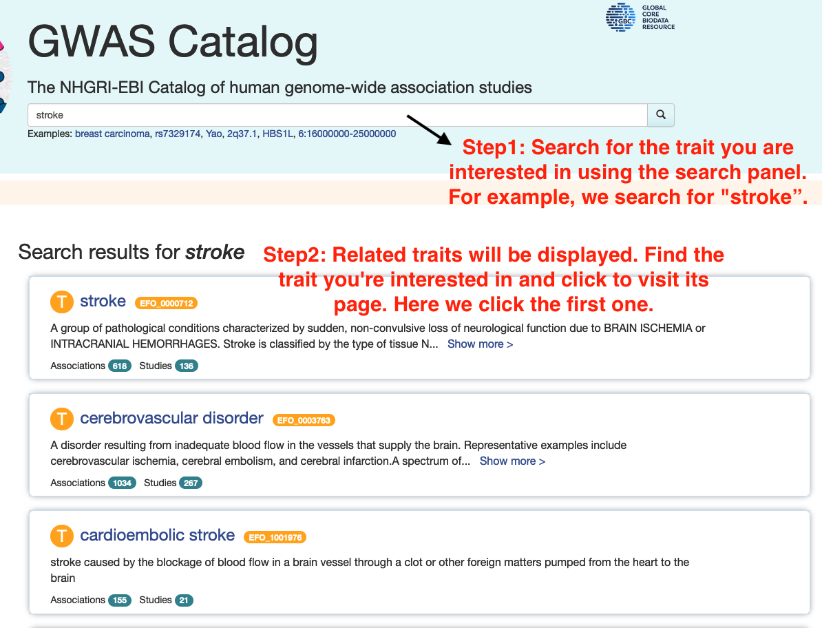
Step 1: Searching for the Trait

  • Go to the GWAS Catalog's search panel.
  • Enter the name or description of the phenotype or disease you're interested in.
  • Navigate to the traits page and then find the trait you are interested in.
  • The first instruction figure below gives an example of finding traits related to stroke.

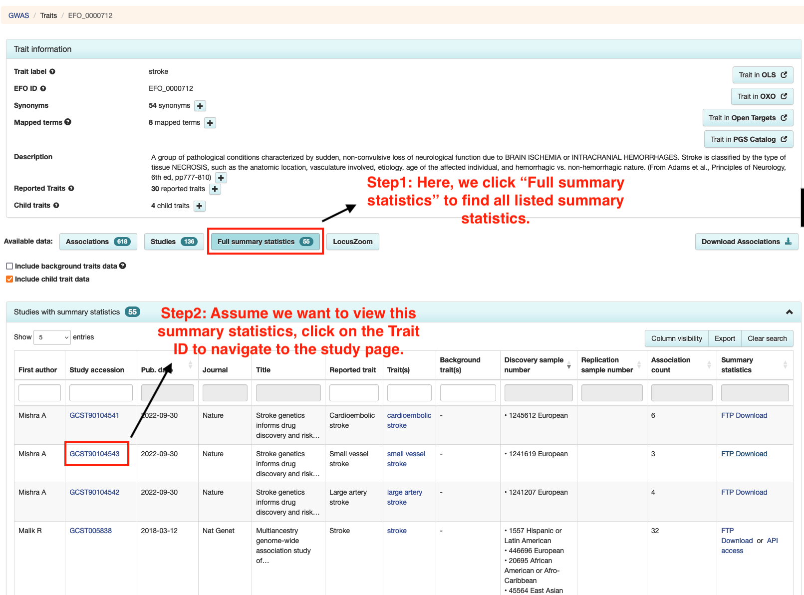
Step 2: Verifying Data Availability

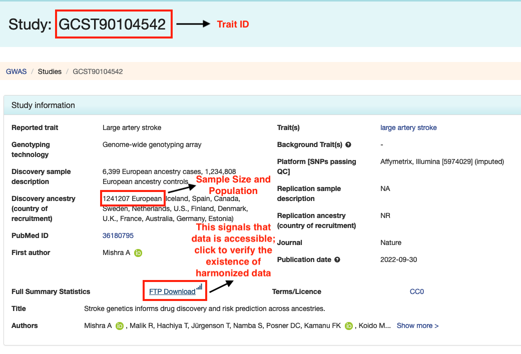
  • Navigate to the study page for your chosen trait, which will be labeled with "Study: [Trait ID]". This page will provide important details like sample size and population, which are necessary for your query.
  • On the studies page, look for the "Full Summary Statistics" section.
  • If there's an "FTP Download" link, this indicates that the original data is available.
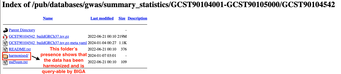
  • Click this link to check if the data has been harmonized. A harmonized dataset will have a "harmonised" folder on the FTP site, indicating it's ready for querying with BIGA.
  • The second instruction figure below will help you identify the "FTP Download" link and the "harmonised" folder.

Step 3: Confirming the trait is query-able by BIGA

  • In the table below, we list all available summary statistics that is query-able by BIGA.
  • Search this table using the Trait ID from Step 1.
  • If your trait is listed, it confirms that the data can be queried using BIGA.

Note: This table is updated daily at 5:30am EST.

Index	Trait ID	GWAS Catalog Link

1.7 Query Data from IEU OpenGWAS

To simplify and clarify the steps for querying summary statistics data from the IEU OpenGWAS, we can break down the process into two steps:

Step 1: Searching for the Trait

  • Go to the IEU OpenGWAS search panel as shown in the first instruction figure below.
  • At the section of Trait contain, enter the name or description of the phenotype or disease you're interested in.
  • Navigate to the data page for your chosen trait, which will be labeled with "Phenotype Name and Dataset: [Trait ID]". This page will provide important details like sample size, population and human genome build version, which are necessary for your query.
  • The data page is similar to the second instruction page below.

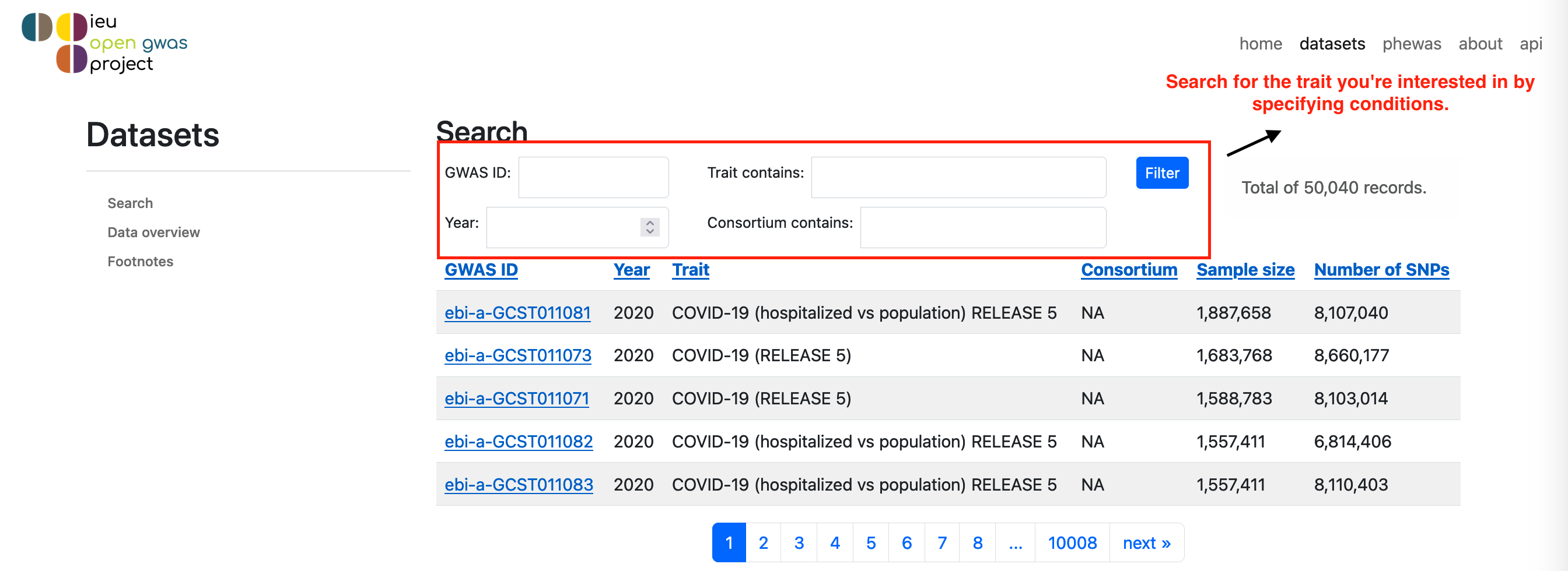
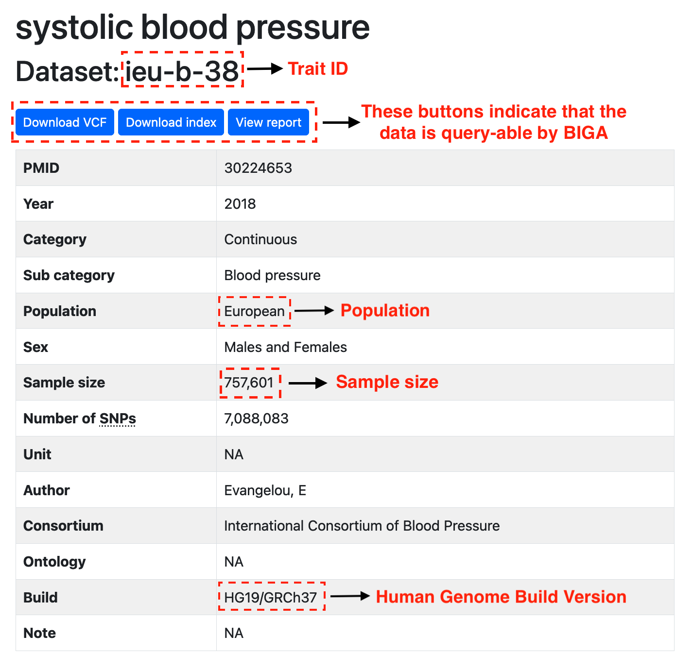
Step 2: Confirming the trait is query-able by BIGA

  • If the "Download VCF" and "Download Index" blue buttons appear, the summary statistics data is query-able by BIGA.
  • Or you can search trait ID or trait description directly using the table below, we list all available summary statistics that is query-able by BIGA.
  • To proceed, enter the trait ID, population, and sample size into the query panel, and select the appropriate human genome build version.

Note: The table is updated monthly at 1:30 AM EST on the 11th day of each month.

Index	Trait ID	Description	Sample Size	Number of SNPs	Population	Build	OpenGWAS LINK

1.8 Query Data from Neale Lab

The Neale Lab datasets have undergone data harmonization. More details about our data processing can be found at UK Biobank (Neale Lab).
The table below lists all the Neale Lab summary statistics data available for querying. To find the data you are interested in, you can directly search by phenotype name or trait ID. In the panel of querying, simply entering the trait ID is sufficient.
For more detailed information about the traits, please refer to Neale Lab's website.

Index	Trait ID	Phenotype

2. Curated Dataset

2.1 Brain and Organ Imaging Traits

Description

BIG-KP is a knowledge portal dedicated to the study of various structural and functional imaging traits of the human brain and other organs. This dataset includes seven distinct sections:
1. Regional brain volumes (n = 101)
2. Diffusion tensor imaging (DTI) parameters (n =110)
3. Resting-state fMRI (rfMRI) traits (n = 1080)
4. Task-related fMRI (tfMRI) traits (n = 919)
5. Regional rfMRI amplitude traits (n= 360)
6. Cardiac imaging traits (n =82)
Trait descriptions can be downloaded here.

Reference

For more information, please visit BIG-KP.

Data Processing

Harmonized by BIGA, the original files have a header with columns CHR, SNP, POS, A1, A2, N, AF1, BETA, SE, P where position is based on the GRCh37 version. These columns are reinterpreted in BIGA's format as chr, snp, position, a1, a2, n, eaf, beta, se, pvalue. Since the snp column is provided, BIGA maps chromosomes and positions by referring to the latest dbSNP build 156 version file when the snp is the same. Next, BIGA infers the orientation (forward or reverse) of palindromic variants by randomly selecting 5% of variants for each chromosome separately, as shown in the log file.

             
Chromosome 1: Forward strand rate: 0.998836, Reverse strand rate: 0.001164
Chromosome 2: Forward strand rate: 0.999861, Reverse strand rate: 0.000139
Chromosome 3: Forward strand rate: 0.999919, Reverse strand rate: 8.1e-05
Chromosome 4: Forward strand rate: 1.0, Reverse strand rate: 0.0
Chromosome 5: Forward strand rate: 1.0, Reverse strand rate: 0.0
Chromosome 6: Forward strand rate: 0.996204, Reverse strand rate: 0.003796
Chromosome 7: Forward strand rate: 0.998482, Reverse strand rate: 0.001518
Chromosome 8: Forward strand rate: 0.999525, Reverse strand rate: 0.000475
Chromosome 9: Forward strand rate: 0.998611, Reverse strand rate: 0.001389
Chromosome 10: Forward strand rate: 0.994752, Reverse strand rate: 0.005248
Chromosome 11: Forward strand rate: 0.994062, Reverse strand rate: 0.005938
Chromosome 12: Forward strand rate: 0.999817, Reverse strand rate: 0.000183
Chromosome 13: Forward strand rate: 1.0, Reverse strand rate: 0.0
Chromosome 14: Forward strand rate: 1.0, Reverse strand rate: 0.0
Chromosome 15: Forward strand rate: 0.993571, Reverse strand rate: 0.006429
Chromosome 16: Forward strand rate: 1.0, Reverse strand rate: 0.0
Chromosome 17: Forward strand rate: 0.99989, Reverse strand rate: 0.00011
Chromosome 18: Forward strand rate: 1.0, Reverse strand rate: 0.0
Chromosome 19: Forward strand rate: 1.0, Reverse strand rate: 0.0
Chromosome 20: Forward strand rate: 1.0, Reverse strand rate: 0.0
Chromosome 21: Forward strand rate: 1.0, Reverse strand rate: 0.0
Chromosome 22: Forward strand rate: 1.0, Reverse strand rate: 0.0
Overall Forward strand rate: 0.998702, Reverse strand rate:0.001298

The script above is the log file of ukb_phase1to3_roi_volume101_june_2020_pheno_9 trait (one trait from the Regional brain volumes group), it's observed that the forward strand rate is above 99%. Therefore, palindromic variants are inferred to be on the forward strand.

             
Chromosome 6, Harmonization summary:
Counter({'Forward strand; Correct orientation; Already harmonised': 380854, 'Forward strand; Flipped orientation; Requires harmonisation': 86197, 'Palindromic; Assume forward strand; Correct orientation; Already harmonised': 67744, 'Palindromic; Assume forward strand; Flipped orientation; Requires harmonisation': 15806, 'Reverse strand; Correct orientation; Already harmonised': 1193, 'Reverse strand; Flipped orientation; Requires harmonisation': 234})

The above is the log file that summarizes the result of chromosome 6 during the harmonization.
Forward strand; Correct orientation; Already harmonised: 380854. It indicates that 380854 SNPs are on the forward DNA strand and are already in the correct orientation. They do not require any further harmonization.
Forward strand; Flipped orientation; Requires harmonisation: 86197. This indicates 86199 SNPs on the forward strand in a flipped orientation. Therefore, BIGA will invert beta,

odds
            ratio

, z-score if provided.
Palindromic; Assume forward strand; Correct orientation; Already harmonised: 67744. This means it's assumed they are on the forward strand and are in the correct orientation, so no further harmonization is needed.
Palindromic; Assume forward strand; Flipped orientation; Requires harmonisation: 15806. This means it's assumed they are on the forward strand but are in the flipped orientation. BIGA will invert beta, odds ratio, z-score if provided.
Reverse strand; Correct orientation; Already harmonised': 1193 This means that 1193 SNPs are on reverse strand but are in the correct orientation as per the reference. They are already harmonized, so BIGA will keep the records.
Reverse strand; Flipped orientation; Requires harmonisation: 234.These 234 SNPs are on the reverse strand and have a flipped orientation, which require harmonization. BIGA will invert beta, odds ratio, z-score if provided.

The harmonization of each chromosome is performed in parallel to save time. After harmonization, BIGA combines each chromosome and sorts harmonized data based on chr and position column. To accommodate the requirements of LDSC, LAVA, Popcorn, and SumHer for a human genome version of GRCh37, BIGA converts the position data from GRCh38 to GRCh37. Then, we get the unified format of input file in BIGA.

2.2 UK Biobank (Neale Lab)

Description

The Neale Lab dataset includes imputed genotypes from HRC plus UK10K & 1000 Genomes reference panels released by UK Biobank in March 2018. This dataset includes 4347 phenotypes categorized under the 'both_sexes' classification and excludes traits marked with an 'pending' status in md5s.
Phenotype description can be downloaded here.

Reference

For more information, please visit Neale Lab.

Data Processing

Harmonized by BIGA, the original files have a header with columns CHR, BP, A1, A2, N, EAF, BETA, SE, P where position is based on the GRCh37 version. These columns are reinterpreted in BIGA's format as chr,position, a1, a2, n, eaf, beta, se, pvalue. Without a snp column provided, the snp column is retrieved during the harmonization step. BIGA maps GRCh37 to GRCh38 locations using a liftover chainfile from UCSC, as the reference file dbSNP build 156 version is built on GRCh38 version. Next, BIGA infers the orientation (forward or reverse) of palindromic variants by randomly selecting 5% of variants for each chromosome separately, as shown in the log file.

             
Chromosome 1: Forward strand rate: 0.999728, Reverse strand rate: 0.000272
Chromosome 2: Forward strand rate: 1.0, Reverse strand rate: 0.0
Chromosome 3: Forward strand rate: 0.999973, Reverse strand rate: 2.7e-05
Chromosome 4: Forward strand rate: 1.0, Reverse strand rate: 0.0
Chromosome 5: Forward strand rate: 1.0, Reverse strand rate: 0.0
Chromosome 6: Forward strand rate: 0.999323, Reverse strand rate: 0.000677
Chromosome 7: Forward strand rate: 0.9998, Reverse strand rate: 0.0002
Chromosome 8: Forward strand rate: 0.999858, Reverse strand rate: 0.000142
Chromosome 9: Forward strand rate: 0.999733, Reverse strand rate: 0.000267
Chromosome 10: Forward strand rate: 0.999042, Reverse strand rate: 0.000958
Chromosome 11: Forward strand rate: 0.999109, Reverse strand rate: 0.000891
Chromosome 12: Forward strand rate: 1.0, Reverse strand rate: 0.0
Chromosome 13: Forward strand rate: 1.0, Reverse strand rate: 0.0
Chromosome 14: Forward strand rate: 1.0, Reverse strand rate: 0.0
Chromosome 15: Forward strand rate: 0.999096, Reverse strand rate: 0.000904
Chromosome 16: Forward strand rate: 1.0, Reverse strand rate: 0.0
Chromosome 17: Forward strand rate: 0.99986, Reverse strand rate: 0.00014
Chromosome 18: Forward strand rate: 1.0, Reverse strand rate: 0.0
Chromosome 19: Forward strand rate: 1.0, Reverse strand rate: 0.0
Chromosome 20: Forward strand rate: 1.0, Reverse strand rate: 0.0
Chromosome 21: Forward strand rate: 1.0, Reverse strand rate: 0.0
Chromosome 22: Forward strand rate: 1.0, Reverse strand rate: 0.0
Overall Forward strand rate: 0.999778, Reverse strand rate:0.000222

The script above is the log file of Z47.gwas.imputed_v3.both_sexes trait (one trait from the Neale Lab group), it can be observed that the forward strand rate is above 99%. Therefore, palindromic variants are inferred to be on the forward strand.

             
Chromosome 6, Harmonization summary:
Counter({'Forward strand; Correct orientation; Already harmonised': 684193, 'Palindromic; Assume forward strand; Correct orientation; Already harmonised': 121370, 'Forward strand; Flipped orientation; Requires harmonisation': 1043, 'Palindromic; Assume forward strand; Flipped orientation; Requires harmonisation': 216, 'Reverse strand; Correct orientation; Already harmonised': 174, 'Reverse strand; Flipped orientation; Requires harmonisation': 143})

The above is the log file that summarizes the result of chromosome 6 during the harmonization.
Forward strand; Correct orientation; Already harmonised: 684193. It indicates that 684193 SNPs are on the forward DNA strand and are already in the correct orientation. They do not require any further harmonization.
Palindromic; Assume forward strand; Correct orientation; Already harmonised: 121370. This means that they are assumed to be on the forward strand and are in the correct orientation, so no further harmonization is needed.
Forward strand; Flipped orientation; Requires harmonisation: 1043. This indicates 1043 SNPs on the forward strand in a flipped orientation. Therefore, BIGA will invert beta,

odds
            ratio

, z-score if provided.
Palindromic; Assume forward strand; Flipped orientation; Requires harmonisation: 216. 216 SNPs fall into this category. This means that they are assumed to be on the forward strand but are in the flipped orientation. BIGA will invert beta, odds ratio, z-score if provided.
Reverse strand; Correct orientation; Already harmonised': 174 This means that 174 SNPs are on reverse strand but are in the correct orientation as per the reference. They are already harmonized. BIGA will keep the records.
Reverse strand; Flipped orientation; Requires harmonisation: 143.These 143 SNPs are on the reverse strand and have a flipped orientation, which require harmonization. BIGA will invert beta, odds ratio, z-score if provided.

Each chromosome harmonization is performed in parallel to save time. After harmonization, BIGA combines each chromosome and sorts harmonized data based on chr and position column. To accommodate the requirements of LDSC, LAVA, Popcorn, and SumHer, which all require a human genome version of GRCh37, BIGA converts the position data from GRCh38 to GRCh37. Then, we get the unified format of input file in BIGA.

2.3 UKB Oxford Brain Imaging Traits

Description

The UKB Oxford Brain Imaging Traits is a collection of neuroimaging data traits derived from the UK Biobank. This dataset includes five distinct sections:
1. Structural MRI (SMRI, n=1437)
2. Difussion MRI (dMRI, n=675)
3. Task functional MRI (tfMRI, n=16)
4. Resting functional MRI (rfMRI, amplitude, n=76)
5. Resting functional MRI (rfMRI, functional connectivity, n=1701)

Trait descriptions can be downloaded here.

Reference

For more information, please visit UKB Oxford.

Data Processing

Harmonized by BIGA, the original files have a header with columns CHR,SNP, POS, A1, A2, N, AF1, BETA, SE, P where position is based on the GRCh37 version. These columns are reinterpreted in BIGA's format as chr, snp, position, a1, a2, n, eaf, beta, se, pvalue. With the snp column provided, BIGA maps snp to chromosome and position by referencing the latest reference file. Next, BIGA infers the orientation (forward or reverse) of palindromic variants by randomly selecting 5% of variants for each chromosome separately, as shown in the log file.

             
Chromosome 1: Forward strand rate: 0.998876, Reverse strand rate: 0.001124
Chromosome 2: Forward strand rate: 0.999965, Reverse strand rate: 3.5e-05
Chromosome 3: Forward strand rate: 1.0, Reverse strand rate: 0.0
Chromosome 4: Forward strand rate: 1.0, Reverse strand rate: 0.0
Chromosome 5: Forward strand rate: 1.0, Reverse strand rate: 0.0
Chromosome 6: Forward strand rate: 0.996888, Reverse strand rate: 0.003112
Chromosome 7: Forward strand rate: 0.99783, Reverse strand rate: 0.00217
Chromosome 8: Forward strand rate: 0.99926, Reverse strand rate: 0.00074
Chromosome 9: Forward strand rate: 0.998916, Reverse strand rate: 0.001084
Chromosome 10: Forward strand rate: 0.995177, Reverse strand rate: 0.004823
Chromosome 11: Forward strand rate: 0.994628, Reverse strand rate: 0.005372
Chromosome 12: Forward strand rate: 0.999821, Reverse strand rate: 0.000179
Chromosome 13: Forward strand rate: 1.0, Reverse strand rate: 0.0
Chromosome 14: Forward strand rate: 1.0, Reverse strand rate: 0.0
Chromosome 15: Forward strand rate: 0.994196, Reverse strand rate: 0.005804
Chromosome 16: Forward strand rate: 1.0, Reverse strand rate: 0.0
Chromosome 17: Forward strand rate: 1.0, Reverse strand rate: 0.0
Chromosome 18: Forward strand rate: 1.0, Reverse strand rate: 0.0
Chromosome 19: Forward strand rate: 1.0, Reverse strand rate: 0.0
Chromosome 20: Forward strand rate: 1.0, Reverse strand rate: 0.0
Chromosome 21: Forward strand rate: 1.0, Reverse strand rate: 0.0
Chromosome 22: Forward strand rate: 0.999575, Reverse strand rate: 0.000425
Overall Forward strand rate: 0.998788, Reverse strand rate:0.001212

The script above is the log file of ukb_smith_dMRI_2_imputed_pheno9 trait (one trait from the dMRI group of UKB Oxford), it's observed that the forward strand rate is above 99%. Therefore, palindromic variants are inferred to be on the forward strand.

             
Chromosome 6, Harmonization summary:
Counter({'Forward strand; Correct orientation; Already harmonised': 380854, 'Forward strand; Flipped orientation; Requires harmonisation': 86199, 'Palindromic; Assume forward strand; Correct orientation; Already harmonised': 67743, 'Palindromic; Assume forward strand; Flipped orientation; Requires harmonisation': 15807, 'Reverse strand; Correct orientation; Already harmonised': 1193, 'Reverse strand; Flipped orientation; Requires harmonisation': 234})

The above is the log file that summarizes the result of chromosome 6 during the harmonization.
Forward strand; Correct orientation; Already harmonised: 380854. It indicates that 380854 SNPs are on the forward DNA strand and are already in the correct orientation. They do not require any further harmonization.
Forward strand; Flipped orientation; Requires harmonisation: 86199 This means 86199 SNPs on the forward strand in a flipped orientation. Therefore, BIGA will invert beta,

odds
            ratio

, z-score if provided.
Palindromic; Assume forward strand; Correct orientation; Already harmonised: 67743. This means it's assumed they are on the forward strand and are in the correct orientation, so no further harmonization is needed.
Palindromic; Assume forward strand; Flipped orientation; Requires harmonisation: 15807. This means it's assumed they are on the forward strand but are in the flipped orientation. BIGA will invert beta, odds ratio, z-score if provided.
Reverse strand; Correct orientation; Already harmonised': 1193 This means that 1193 SNPs are on reverse strand but are in the correct orientation as per the reference. They are already harmonized. BIGA will keep the records.
Reverse strand; Flipped orientation; Requires harmonisation: 234.These 234 SNPs are on the reverse strand and have a flipped orientation, which require harmonization. BIGA will invert beta, odds ratio, z-score if provided.

Each chromosome harmonization is performed in parallel to save time. After harmonization, BIGA combines each chromosome and sorts harmonized data based on chr and position column. To accommodate the requirements of LDSC, LAVA, Popcorn, and SumHer, which all require a human genome version of GRCh37, BIGA converts the position data from GRCh38 to GRCh37. Then, we get the unified format of input file in BIGA.

2.4 Biobank Japan

Description

The Biobank Japan project is a large-scale biobank that collects genetic, clinical, and lifestyle information from a cohort of Japanese individuals. This dataset includes 177 phenotypes.

Phenotype descriptions can be downloaded here.

Reference

For more information, please visit Biobank Japan.

Data Processing

Harmonized by BIGA, the original files have a header with columns CHR,SNPID, POS, Allele1, Allele2, N, AF_Allele2, BETA, SE, p.value where position is based on the GRCh37 version. Please note that Allele2 is the effect allele. These columns are reinterpreted in BIGA's format as chr, snp, position, a2, a1, n, eaf, beta, se, pvalue. With the snp column provided, BIGA maps snp to chromosome and position by referencing the latest reference file. Next, BIGA infers the orientation (forward or reverse) of palindromic variants by randomly selecting 5% of variants for each chromosome separately, as shown in the log file.

             
Chromosome 1: Forward strand rate: 0.999125, Reverse strand rate: 0.000875
Chromosome 2: Forward strand rate: 0.999894, Reverse strand rate: 0.000106
Chromosome 3: Forward strand rate: 0.99997, Reverse strand rate: 3e-05
Chromosome 4: Forward strand rate: 1.0, Reverse strand rate: 0.0
Chromosome 5: Forward strand rate: 1.0, Reverse strand rate: 0.0
Chromosome 6: Forward strand rate: 0.997778, Reverse strand rate: 0.002222
Chromosome 7: Forward strand rate: 0.998396, Reverse strand rate: 0.001604
Chromosome 8: Forward strand rate: 0.999838, Reverse strand rate: 0.000162
Chromosome 9: Forward strand rate: 1.0, Reverse strand rate: 0.0
Chromosome 10: Forward strand rate: 0.997203, Reverse strand rate: 0.002797
Chromosome 11: Forward strand rate: 0.998023, Reverse strand rate: 0.001977
Chromosome 12: Forward strand rate: 0.999909, Reverse strand rate: 9.1e-05
Chromosome 13: Forward strand rate: 1.0, Reverse strand rate: 0.0
Chromosome 14: Forward strand rate: 1.0, Reverse strand rate: 0.0
Chromosome 15: Forward strand rate: 0.99764, Reverse strand rate: 0.00236
Chromosome 16: Forward strand rate: 1.0, Reverse strand rate: 0.0
Chromosome 17: Forward strand rate: 1.0, Reverse strand rate: 0.0
Chromosome 18: Forward strand rate: 1.0, Reverse strand rate: 0.0
Chromosome 19: Forward strand rate: 1.0, Reverse strand rate: 0.0
Chromosome 20: Forward strand rate: 1.0, Reverse strand rate: 0.0
Chromosome 21: Forward strand rate: 1.0, Reverse strand rate: 0.0
Chromosome 22: Forward strand rate: 0.999809, Reverse strand rate: 0.000191
Overall Forward strand rate: 0.999342, Reverse strand rate:0.000658

The script above is the log file of GWASsummary_Zoster_Japanese_SakaueKanai2020 trait (one trait from the Biobank Japan), it's observed that the forward strand rate is above 99%. Therefore, palindromic variants are inferred to be on the forward strand.

             
Chromosome 6, Harmonization summary:
Counter({'Forward strand; Correct orientation; Already harmonised': 628517, 'Palindromic; Assume forward strand; Correct orientation; Already harmonised': 103469, 'Reverse strand; Correct orientation; Already harmonised': 1256, 'Forward strand; Flipped orientation; Requires harmonisation': 779, 'Palindromic; Assume forward strand; Flipped orientation; Requires harmonisation': 356, 'Reverse strand; Flipped orientation; Requires harmonisation': 25})

The above is the log file that summarizes the result of chromosome 6 during the harmonization.
Forward strand; Correct orientation; Already harmonised: 628517. It indicates that 628517 SNPs are on the forward DNA strand and are already in the correct orientation. They do not require any further harmonization.
Palindromic; Assume forward strand; Correct orientation; Already harmonised: 103469. This means it's assumed they are on the forward strand and are in the correct orientation, so no further harmonization is needed.
Reverse strand; Correct orientation; Already harmonised': 1256 This means that 1256 SNPs are on reverse strand but are in the correct orientation as per the reference. They are already harmonized. BIGA will keep the records.
Forward strand; Flipped orientation; Requires harmonisation: 779 This means 779 SNPs on the forward strand in a flipped orientation. Therefore, BIGA will invert beta, odds ratio, z-score if provided.
Palindromic; Assume forward strand; Flipped orientation; Requires harmonisation: 356. This means it's assumed they are on the forward strand but are in the flipped orientation. BIGA will invert beta, odds ratio, z-score if provided.
Reverse strand; Flipped orientation; Requires harmonisation: 25. These 25 SNPs are on the reverse strand and have a flipped orientation, which require harmonization. BIGA will invert beta, odds ratio, z-score if provided.

Each chromosome harmonization is performed in parallel to save time. After harmonization, BIGA combines each chromosome and sorts harmonized data based on chr and position column. To accommodate the requirements of LDSC, LAVA, Popcorn, and SumHer, which all require a human genome version of GRCh37, BIGA converts the position data from GRCh38 to GRCh37. Then, we get the unified format of input file in BIGA.

2.5 UKB-PPP European Protein GWAS

Description

The UKB-PPP European Protein GWAS dataset refers to a collection of GWAS summary statistics of the protein expressions within a European population. This dataset includes 2940 proteins.

Trait descriptions can be downloaded here.

Reference

For more information, please visit UKB-PPP.

Data Processing

Harmonized by BIGA, the original files have a header with columns CHROM,POS, ALLELE0, ALLELE1, N, A1FREQ, BETA, SE, P where position is based on the GRCh37 version. Please note that ALLELE1 is the effect allele. These columns are reinterpreted in BIGA's format as chr, position, a2, a1, n, eaf, beta, se, pvalue. Without a snp column provided, the snp column is retrieved during the harmonization step. BIGA maps hg19 to hg38 locations using a liftover chainfile from UCSC, as the reference file dbSNP build 156 version is built on GRCh38 version. Next, BIGA infers the orientation (forward or reverse) of palindromic variants by randomly selecting 5% of variants for each chromosome separately, as shown in the log file.

             
Chromosome 1: Forward strand rate: 0.999762, Reverse strand rate: 0.000238
Chromosome 2: Forward strand rate: 0.99998, Reverse strand rate: 2e-05
Chromosome 3: Forward strand rate: 1.0, Reverse strand rate: 0.0
Chromosome 4: Forward strand rate: 1.0, Reverse strand rate: 0.0
Chromosome 5: Forward strand rate: 1.0, Reverse strand rate: 0.0
Chromosome 6: Forward strand rate: 0.999208, Reverse strand rate: 0.000792
Chromosome 7: Forward strand rate: 0.999884, Reverse strand rate: 0.000116
Chromosome 8: Forward strand rate: 0.999969, Reverse strand rate: 3.1e-05
Chromosome 9: Forward strand rate: 0.999528, Reverse strand rate: 0.000472
Chromosome 10: Forward strand rate: 0.998169, Reverse strand rate: 0.001831
Chromosome 11: Forward strand rate: 0.999345, Reverse strand rate: 0.000655
Chromosome 12: Forward strand rate: 1.0, Reverse strand rate: 0.0
Chromosome 13: Forward strand rate: 1.0, Reverse strand rate: 0.0
Chromosome 14: Forward strand rate: 1.0, Reverse strand rate: 0.0
Chromosome 15: Forward strand rate: 0.999345, Reverse strand rate: 0.000655
Chromosome 16: Forward strand rate: 1.0, Reverse strand rate: 0.0
Chromosome 17: Forward strand rate: 1.0, Reverse strand rate: 0.0
Chromosome 18: Forward strand rate: 1.0, Reverse strand rate: 0.0
Chromosome 19: Forward strand rate: 1.0, Reverse strand rate: 0.0
Chromosome 20: Forward strand rate: 1.0, Reverse strand rate: 0.0
Chromosome 21: Forward strand rate: 1.0, Reverse strand rate: 0.0
Chromosome 22: Forward strand rate: 1.0, Reverse strand rate: 0.0
Overall Forward strand rate: 0.999754, Reverse strand rate:0.000246

The script above is the log file of ZPR1_O75312_OID30801_v1_Neurology_II trait (one trait from the UKB-PPP), it is observed that the forward strand rate is above 99%. Therefore, palindromic variants are inferred to be on the forward strand.

             
Chromosome 6, Harmonization summary:
Counter({'Forward strand; Correct orientation; Already harmonised': 784340, 'Palindromic; Assume forward strand; Correct orientation; Already harmonised': 139553, 'Forward strand; Flipped orientation; Requires harmonisation': 932, 'Reverse strand; Correct orientation; Already harmonised': 205, 'Palindromic; Assume forward strand; Flipped orientation; Requires harmonisation': 187, 'Reverse strand; Flipped orientation; Requires harmonisation': 178})

The above is the log file that summarizes the result of chromosome 6 during the harmonization.
Forward strand; Correct orientation; Already harmonised: 784340. It indicates that 784340 SNPs are on the forward DNA strand and are already in the correct orientation. They do not require any further harmonization.
Palindromic; Assume forward strand; Correct orientation; Already harmonised: 139553. This means it's assumed they are on the forward strand and are in the correct orientation, so no further harmonization is needed.
Forward strand; Flipped orientation; Requires harmonisation: 932 This means 932 SNPs on the forward strand in a flipped orientation. Therefore, BIGA will invert beta, odds ratio, z-score if provided.
Reverse strand; Correct orientation; Already harmonised: 205. A small number of SNPs (205) are on the reverse DNA strand but are in the correct orientation as per the reference. They are already harmonized. BIGA will keep the records.
Palindromic; Assume forward strand; Flipped orientation; Requires harmonisation: 187. This means it's assumed they are on the forward strand but are in the flipped orientation. BIGA will invert beta, odds ratio, z-score if provided.
Reverse strand; Flipped orientation; Requires harmonisation: 178. 178 SNPs fall into this category, where they are on the reverse strand and have a flipped orientation. These require harmonization. BIGA will invert beta, odds ratio, z-score if provided.

Each chromosome harmonization is performed in parallel to save time. After harmonization, BIGA combines each chromosome and sorts harmonized data based on chr and position column. To accommodate the requirements of LDSC, LAVA, Popcorn, and SumHer, which all require a human genome version of GRCh37, BIGA converts the position data from GRCh38 to GRCh37. Then, we get the unified format of input file in BIGA.

2.6 FinnGen

Description

The FinnGen dataset is a large-scale genetic research project combining Finnish biobank data with comprehensive health records. This dataset includes 303 selected diseases with the number of case larger than 10,000.

Disease descriptions can be downloaded here.

Reference

For more information, please visit FinnGen.

Data Processing

Harmonized by BIGA, the original files have a header with columns CHR,SNP, POS, effect_allele, other_allele, N, effect_allele_freqency, beta, se, P where position is based on the GRCh37 version. These columns are reinterpreted in BIGA's format as chr, snp, position, a1, a2, n, eaf, beta, se, pvalue. With the snp column provided, BIGA maps snp to chromosome and position by referencing the latest reference file. Next, BIGA infers the orientation (forward or reverse) of palindromic variants by randomly selecting 5% of variants for each chromosome separately, as shown in the log file.

             
Chromosome 1: Forward strand rate: 0.999709, Reverse strand rate: 0.000291
Chromosome 2: Forward strand rate: 1.0, Reverse strand rate: 0.0
Chromosome 3: Forward strand rate: 1.0, Reverse strand rate: 0.0
Chromosome 4: Forward strand rate: 1.0, Reverse strand rate: 0.0
Chromosome 5: Forward strand rate: 1.0, Reverse strand rate: 0.0
Chromosome 6: Forward strand rate: 1.0, Reverse strand rate: 0.0
Chromosome 7: Forward strand rate: 0.999907, Reverse strand rate: 9.3e-05
Chromosome 8: Forward strand rate: 1.0, Reverse strand rate: 0.0
Chromosome 9: Forward strand rate: 1.0, Reverse strand rate: 0.0
Chromosome 10: Forward strand rate: 0.999918, Reverse strand rate: 8.2e-05
Chromosome 11: Forward strand rate: 1.0, Reverse strand rate: 0.0
Chromosome 12: Forward strand rate: 1.0, Reverse strand rate: 0.0
Chromosome 13: Forward strand rate: 1.0, Reverse strand rate: 0.0
Chromosome 14: Forward strand rate: 1.0, Reverse strand rate: 0.0
Chromosome 15: Forward strand rate: 1.0, Reverse strand rate: 0.0
Chromosome 16: Forward strand rate: 1.0, Reverse strand rate: 0.0
Chromosome 17: Forward strand rate: 0.999802, Reverse strand rate: 0.000198
Chromosome 18: Forward strand rate: 1.0, Reverse strand rate: 0.0
Chromosome 19: Forward strand rate: 1.0, Reverse strand rate: 0.0
Chromosome 20: Forward strand rate: 1.0, Reverse strand rate: 0.0
Chromosome 21: Forward strand rate: 1.0, Reverse strand rate: 0.0
Chromosome 22: Forward strand rate: 0.999707, Reverse strand rate: 0.000293
Overall Forward strand rate: 0.999958, Reverse strand rate:4.2e-05

The script above is the log file of finngen_R9_Z21_PROCREATIVE_MANAG_GRCh37_CrossMap trait (one trait from the FinnGen), it's observed that the forward strand rate is above 99%. Therefore, palindromic variants are inferred to be on the forward strand.

             
Chromosome 6, Harmonization summary:
Counter({'Forward strand; Correct orientation; Already harmonised': 945824, 'Palindromic; Assume forward strand; Correct orientation; Already harmonised': 166105, 'Forward strand; Flipped orientation; Requires harmonisation': 45, 'Palindromic; Assume forward strand; Flipped orientation; Requires harmonisation': 6, 'Reverse strand; Correct orientation; Already harmonised': 5})

The above is the log file that summarizes the result of chromosome 6 during the harmonization.
Forward strand; Correct orientation; Already harmonised: 945824. It indicates that 945824 SNPs are on the forward DNA strand and are already in the correct orientation. They do not require any further harmonization.
Palindromic; Assume forward strand; Correct orientation; Already harmonised: 166105. This means it's assumed they are on the forward strand and are in the correct orientation, so no further harmonization is needed.
Forward strand; Flipped orientation; Requires harmonisation: 45 This means 45 SNPs on the forward strand in a flipped orientation. Therefore, BIGA will invert beta, odds ratio, z-score if provided.
Palindromic; Assume forward strand; Flipped orientation; Requires harmonisation: 6. This means it's assumed they are on the forward strand but are in the flipped orientation. BIGA will invert beta, odds ratio, z-score if provided.
Reverse strand; Correct orientation; Already harmonised: 5. A small number of SNPs (306) are on the reverse DNA strand but are in the correct orientation as per the reference. They are already harmonized. BIGA will keep the records.

Each chromosome harmonization is performed in parallel to save time. After harmonization, BIGA combines each chromosome and sorts harmonized data based on chr and position column. To accommodate the requirements of LDSC, LAVA, Popcorn, and SumHer, which all require a human genome version of GRCh37, BIGA converts the position data from GRCh38 to GRCh37. Then, we get the unified format of input file in BIGA.

2.7 PGC (Psychiatric Genomics Consortium) and Other Brain Disorders

Description

The PGC dataset represents a comprehensive collection of genetic and clinical data focused on psychiatric disorders. In addition, we also included a few brain disorders such as Alzheimer's disease, Stroke and its subtypes, and Depression. This dataset currently contains 24 phenotypes.
Phenotype descriptions can be downloaded here.

Reference

For more information about PGC, please visit the PGC website.

Data Processing

Partially harmonized by BIGA due to missing specific columns in some traits. Harmonized traits include ADHD, several bipolar disorder indices (pgc_bip2021_al, pgc_bip2021_BDI, pgc_bip2021_BDII), depression-related traits (depression_pgc_ukb, pts_eur_freeze2_overall), hoarding2022, and a series of traits related to schizophrenia (PGC3_SCZ_wave3, depression, GCST90104539-43, GCST90027158). Traits that remain unharmonized are TS_Oct2018, several opioid exposure comparisons within European ancestry cohorts, substance use disorder indices (CUD_EUR_full_public_11.14.2020, pgc_alcdep.eur_discovery.aug2018_release), ocd_aug2017, autism spectrum disorder traits (iPSYCH-PGC_ASD_Nov2017), and pgcAN2_2019_07.

2.8 GWAS Catalog

Description

The GWAS Catalog is a comprehensive resource that provides access to a curated collection of GWAS results. This dataset includes 897 traits, curated to include those with substantial sample sizes (the number of case larger than 5,000 for diseases and the sample size larger than 10,000 for traits) . Datasets with high missing rate in beta, odds_ratio, se columns are removed.
Phenotype descriptions can be downloaded here.

Reference

For more information, please visit GWAS Catalog.

Data Processing

These data have been harmonized by GWAS Catalog. BIGA converts the pre-downloaded data into the universal format, incorporating columns snp, chr, position, pvalue, eaf, a1, a2, n, odds_ratio or beta, and se. The harmonized file from the GWAS Catalog might present diverse column names to represent harmonized columns. For instance, beta could be labeled as `hm_beta` or `beta`. BIGA first checks for hm_beta; if absent, it defaults to the beta column.
To accommodate the requirements of LDSC, LAVA, Popcorn, and SumHer, which all require a human genome version of GRCh37, BIGA converts the position from GRCh38 to GRCh37. Then, we get the unified format of input file in BIGA.

2.9 CHIMGEN

Description

The Chinese Imaging Genetics (CHIMGEN) study is a comprehensive neuroimaging genetics cohort in the Chinese population. This dataset includes 44 hippocampal volumetric traits.
Trait descriptions can be downloaded here.

Reference

For more information, please visit CHIMGEN.

Data Processing

Harmonized by BIGA, the original files have a header with columns chr,pos, Other_allele, Effect_allele, af_Effect_allele, beta, se, -log10P, P, N where position is based on the GRCh37 version. pvalue is calculated from -log10P. These columns are reinterpreted in BIGA's format as chr, position, a2, a1, eaf, beta, se, pvalue, n. Without a snp column provided, the snp column is retrieved during the harmonization step. BIGA maps hg19 to hg38 locations using a liftover chainfile from UCSC, as the reference file dbSNP build 156 version is built on GRCh38 version. Next, BIGA infers the orientation (forward or reverse) of palindromic variants by randomly selecting 5% of variants for each chromosome separately, as shown in the log file.

             
Chromosome 1: Forward strand rate: 0.999758, Reverse strand rate: 0.000242
Chromosome 2: Forward strand rate: 0.99998, Reverse strand rate: 2e-05
Chromosome 3: Forward strand rate: 1.0, Reverse strand rate: 0.0
Chromosome 4: Forward strand rate: 1.0, Reverse strand rate: 0.0
Chromosome 5: Forward strand rate: 1.0, Reverse strand rate: 0.0
Chromosome 6: Forward strand rate: 0.999614, Reverse strand rate: 0.000386
Chromosome 7: Forward strand rate: 0.999405, Reverse strand rate: 0.000595
Chromosome 8: Forward strand rate: 0.999934, Reverse strand rate: 6.6e-05
Chromosome 9: Forward strand rate: 0.999876, Reverse strand rate: 0.000124
Chromosome 10: Forward strand rate: 0.998454, Reverse strand rate: 0.001546
Chromosome 11: Forward strand rate: 0.99927, Reverse strand rate: 0.00073
Chromosome 12: Forward strand rate: 0.999929, Reverse strand rate: 7.1e-05
Chromosome 13: Forward strand rate: 1.0, Reverse strand rate: 0.0
Chromosome 14: Forward strand rate: 1.0, Reverse strand rate: 0.0
Chromosome 15: Forward strand rate: 0.998746, Reverse strand rate: 0.001254
Chromosome 16: Forward strand rate: 1.0, Reverse strand rate: 0.0
Chromosome 17: Forward strand rate: 0.999937, Reverse strand rate: 6.3e-05
Chromosome 18: Forward strand rate: 1.0, Reverse strand rate: 0.0
Chromosome 19: Forward strand rate: 1.0, Reverse strand rate: 0.0
Chromosome 20: Forward strand rate: 1.0, Reverse strand rate: 0.0
Chromosome 21: Forward strand rate: 0.999867, Reverse strand rate: 0.000133
Chromosome 22: Forward strand rate: 0.999744, Reverse strand rate: 0.000256
Overall Forward strand rate: 0.999748, Reverse strand rate:0.000252

The script above is the log file of R_subiculum_head trait (one trait from the CHIMGEN), it's observed that the forward strand rate is above 99%. Therefore, palindromic variants are inferred to be on the forward strand.

             
Chromosome 6, Harmonization summary:
Counter({'Forward strand; Correct orientation; Already harmonised': 775133, 'Palindromic; Assume forward strand; Correct orientation; Already harmonised': 144108, 'Forward strand; Flipped orientation; Requires harmonisation': 1035, 'Palindromic; Assume forward strand; Flipped orientation; Requires harmonisation': 216, 'Reverse strand; Correct orientation; Already harmonised': 197, 'Reverse strand; Flipped orientation; Requires harmonisation': 171})

The above is the log file that summarizes the result of chromosome 6 during the harmonization.
Forward strand; Correct orientation; Already harmonised: 775133. It indicates that 775133 SNPs are on the forward DNA strand and are already in the correct orientation. They do not require any further harmonization.
Palindromic; Assume forward strand; Correct orientation; Already harmonised: 144108. This means it's assumed they are on the forward strand and are in the correct orientation, so no further harmonization is needed.
Forward strand; Flipped orientation; Requires harmonisation: 1035 This means 1035 SNPs on the forward strand in a flipped orientation. Therefore, BIGA will invert beta, odds ratio, z-score if provided.
Palindromic; Assume forward strand; Flipped orientation; Requires harmonisation: 216. This means it's assumed they are on the forward strand but are in the flipped orientation. BIGA will invert beta, odds ratio, z-score if provided.
Reverse strand; Correct orientation; Already harmonised: 197. A small number of SNPs (197) are on the reverse DNA strand but are in the correct orientation as per the reference. They are already harmonized. BIGA will keep the records.
Reverse strand; Flipped orientation; Requires harmonisation: 171. These 171 SNPs are on the reverse strand and have a flipped orientation, which require harmonization. BIGA will invert beta, odds ratio, z-score if provided.

Each chromosome harmonization is performed in parallel to save time. After harmonization, BIGA combines each chromosome and sorts harmonized data based on chr and position column. To accommodate the requirements of LDSC, LAVA, Popcorn, and SumHer, which all require a human genome version of GRCh37, BIGA converts the position data from GRCh38 to GRCh37. Then, we get the unified format of input file in BIGA.

3. Analysis Methods

3.1 Massive LDSC Analysis

Reference

LDSC: version 1.0.1

Curated Dataset

BIGA offers 7 European datasets and 2 East Asian datasets for linkage disequilibrium score regression (LDSC) genetic correlation analysis. These datasets include:
1. Brain and Organ Imaging Traits
2. PGC and and Other Brain Disorders
3. FinnGen
4. UK Biobank (Neale Lab)
5. Biobank Japan
6. UKB-Oxford Brain Imaging Traits
7. GWAS Catalog
8. UKB-PPP European Protein GWAS
9. CHIMGEN

Input File Build

The standard input file format in LDSC is .sumstats.gz. This format is achieved using munge_sumstats.py from the LDSC software. The script parameters differ based on columns provided in the input file:
If both beta and odds_ratio are present, BIGA prioritizes beta. The followings are the BIGA's default running script:

python2 $ldsc_path/munge_sumstats.py --sumstats $summary_statistics1 --out $output --merge-alleles $ldsc_path/w_hm3.snplist --chunksize 100000 --ignore 'odds_ratio'

If only one signed summary statistic is present:

python2 $ldsc_path/munge_sumstats.py --sumstats $summary_statistics1 --out $output --merge-alleles $ldsc_path/w_hm3.snplist --chunksize 100000

BIGA's format does not require an INFO column. LDSC used the HapMap3 variants (with the --merge-alleles flag) and the variants in the major histocompatibility complex region were removed. GWAS summary statistics datasets have the sample size column, making the --N flag unnecessary.

Configuration Settings

BIGA offers the option to run LDSC genetic correlation in European GWAS or East Asian GWAS. The LD scores ( used by --w-ld-chr and --ref-ld-chr flags) were from the 1000 Genomes data and were downloaded from LDSC. Specifically:
For European GWAS: Use --w-ld-chr eur_w_ld_chr/ --ref-ld-chr eur_w_ld_chr/
For East Asian GWAS: Use --w-ld-chr eas_ldscores/ --ref-ld-chr eas_ldscores/

Default Script

The script is for running and summarizing the results of LD Score Regression (LDSC).


python2 $ldsc_path/ldsc.py      --ref-ld-chr $ref_chr         --w-ld-chr $w_chr         --out $ldsc_path/log/$job_id/one    --rg $summary_statistics1,$summary_statistics2'ukb_phase1to3_ica_node_may_2022_imputed_pheno10_harmo.sumstats.gz',$summary_statistics2'ukb_phase1to3_ica_node_may_2022_imputed_pheno41_harmo.sumstats.gz',$summary_statistics2'ukb_phase1to3_ica_node_may_2022_imputed_pheno29_harmo.sumstats.gz',...

cd $ldsc_path/log/$job_id/
mkdir less

for file in *log
do
        sed -n -e '/Summary of Genetic Correlation Results/,/Analysis finished/ p' ${file} > less/less_${file}

        awk 'NR>2 && NR<79{print}' less/less_${file} > less/temp.txt ; mv less/temp.txt less/less_${file}
done

The first part involves LDSC execution. ref-ld-chr $ref_chr and --w-ld-chr $w_chr specify the reference LD scores and their weights, which vary by the population.

--out
            $ldsc_path/log/$job_id/one

determines the output directory and filename prefix for the LDSC results for each job. --rg is used to instruct LDSC to calculate genetic correlation. $summary_statistics1 is the path to the input file. $summary_statistics2 is the path prefix of the curated dataset. Each file in this dataset represents different phenotypes, and LDSC will calculate the genetic correlations between the input file and the curated datasets.

The second part summarizes the LDSC results.

sed -n -e '/Summary of Genetic Correlation
            Results/,/Analysis finished/ p' ${file}

: This command extracts a specific section from each log file, starting from where it finds the phrase "Summary of Genetic Correlation Results" and ending at "Analysis finished". This section is then redirected to a new file in the less directory.

awk 'NR>2 &&
            NR<79{print}' less/less_${file}

: This awk command further processes each extracted section, selecting only specific lines (from line 3 to 78), which presumably contain the relevant summarized data. The result is temporarily saved in less/temp.txt. Afterwards, BIGA will save all the results into the database.

3.2 Massive SumHer Analysis

Reference

SumHer: ldak5.2

Curated Dataset

BIGA offers 7 European datasets and 2 East Asian datasets for SumHer genetic correlation analysis. These datasets include:
1. Brain and Organ Imaging Traits
2. PGC and and Other Brain Disorders
3. FinnGen
4. UK Biobank (Neale Lab)
5. Biobank Japan
6. UKB-Oxford Brain Imaging Traits
7. GWAS Catalog
8. UKB-PPP European Protein GWAS
9. CHIMGEN

Input File Build

The standard input file format for SumHer is a text file with a header row. BIGA's unified format meets SumHer's requirements for the input file. Columns such as chr (chromosome), position, a1 (allele 1), a2 (allele 2), n (sample size), and statistical measures like beta or odds_ratio and se (standard error) are extracted from this universal format. These are then transformed into a format suitable for SumHer: chr:position is labeled as Predictor, a1 as A1, a2 as A2, and n remains. The statistical measures are converted into Z statistics, either using beta/se or log(odds_ratio)/se. Additionally, the snp column filters out SNPs that are not part of the HapMap3 dataset (approximately 1.2 million SNPs). After preparing these columns, BIGA removes any duplicate Predictors to retain only the first occurrence and keeps rows with single-character alleles (A, C, G, T).

Configuration Settings

1. Reference Taggings File: SumHer requires a tagging file for estimating genetic correlations. BIGA uses the pre-computed LDAK-Thin Tagging File as recommended in SumHer including LDAK-Thin Tagging File (GBR population, HapMap3 SNPs), LDAK-Thin Tagging File (EAS population, HapMap3 SNPs) for two populations - the GBR (European) and EAS (East Asian) populations.
2. Phenotypic Variance Cutoff: BIGA adheres to SumHer's recommendation and applies a cutoff of 0.01. This means that it removes any predictors that account for more than 1% of the phenotypic variance.
3. Ambiguous Alleles: Since the data is harmonized, ambiguous alleles (A&T or C&G) were aligned with the latest dbsnp 156 reference file. It is not necessary to remove ambiguous alleles, BIGA allows these alleles with the setting

--allow-ambiguous
            YES

.
4. SNP Availability: To address cases where some SNPs in the summary statistics might not be present in the tagging file, BIGA uses the setting --check-sums NO to avoid related errors.

Default Script

The provided script automates the process of genetic correlation analysis using SumHer, working with various datasets:


(arr=("finngen_R9_O15_PREG_OTHER_MAT_DISORD_GRCh37_CrossMap_harmo.txt",...,"finngen_R9_PAIN_GRCh37_CrossMap_harmo.txt")
for trait2 in "${arr[@]}"; do
  out=$sumHer_path/log/$job_id/$trait2
  $sumHer_path/ldak5.2.$envir --summary $summary_statistics1 --summary2 $summary_statistics2/$trait2 --sum-cors $out --tagfile $sumHer_path/ldak.thin.hapmap.$popu.tagging --check-sums NO --allow-ambiguous YES
done) &

(arr=("finngen_R9_M13_ARTHROSIS_KNEE_GRCh37_CrossMap_harmo.txt" ,...,"finngen_R9_E4_LIPOPROT_GRCh37_CrossMap_harmo.txt")
for trait2 in "${arr[@]}"; do
  out=$sumHer_path/log/$job_id/$trait2
  $sumHer_path/ldak5.2.$envir --summary $summary_statistics1 --summary2 $summary_statistics2/$trait2 --sum-cors $out --tagfile $sumHer_path/ldak.thin.hapmap.$popu.tagging --check-sums NO --allow-ambiguous YES
done) &
wait

$summary_statistics1 represents the input summary data, either uploaded or queried by the user. $summary_statistics2 is the directory where BIGA's curated data is stored. $trait2 refers to specific trait filenames from the FinnGen dataset in this case. $popu is a variable indicating the population-specific GWAS dataset, which can be either 'gbr' for the European population or 'eas' for East Asian. The script employs a parallel processing approach, indicated by & at the end of each command. Two arrays of filenames (`arr`) are iterated over, and for each file, a SumHer analysis is conducted using the ldak5.2.$envir command. $envir can either be .mac or .linux depending on the operation system. This command processes both the user's input data and BIGA's curated data, applying the necessary configuration settings, like tagging file selection (--tagfile), allowing ambiguous alleles (--allow-ambiguous YES), and bypassing SNP checks (--check-sums NO). The wait command at the end ensures that all parallel processes are completed before moving on.

3.3 Massive LAVA Analysis

Reference

LAVA: version 0.1.0

Curated Dataset

BIGA offers 7 European datasets for LAVA local genetic correlation analysis. These datasets include:
1. Brain and Organ Imaging Traits
2. PGC and and Other Brain Disorders
3. FinnGen
4. UK Biobank (Neale Lab)
5. UKB-Oxford Brain Imaging Traits
6. GWAS Catalog
7. UKB-PPP European Protein GWAS
In each curated dataset, users currently have the option to select up to 10 traits for running LAVA’s massive analysis.

Input File Build

The standard input file format for LAVA is a text file with a header row. BIGA's unified format meets LAVA's requirements for the input file. Columns including snp, a1,a2,n,beta or odds_ratio,pvalue are extracted from this universal format. These are then transformed into a format suitable for LAVA: snp is labeled as SNP, a1 as A1 and a2 and A2, n as N, beta as BETA, pvalue as P, odds_ratio as OR. Furthermore, the SNPs in the input file are filtered using reference data from Phase 3 of the 1000 Genomes Project. LAVA loci can be defined using genomic coordinates or a list of SNPs, and BIGA uses the same loci definition as LAVA, utilizing the 1000 Genomes Project data (Phase 3, build GRCh37/hg19). Sample overlap file is set to NULL.

Default Script


testPath = trait1_path
testName = t1_name
infoFile = paste('data/',job_id,'/','input.info.txt',sep = "")
sink(infoFile)
cat("phenotype	cases	controls	filename\n")
temp = paste(testName,"NA","NA",testPath,'\n',sep=" ")
cat(temp,append = FALSE)
sink(NULL)
trait1 = process.input(input.info.file=infoFile,
                       sample.overlap.file=NULL,
                       ref.prefix="vignettes/data/ldsc_g1000_eur",phenos=c(t1_name))

In this segment, the script prepares the environment for LAVA analysis. It sets up the path of input summary data and filename for the trait under study (trait1_path and t1_name). The infoFile is a configuration file that details the input file, including cases and controls set to NA, along with their respective filenames. The process.input function is then called to process this input data, considering the reference file from phase 3 of the 1000 Genomes Project (ref.prefix).


 if (n.run>0){
  for (i in 1:n.run) {
    start_time <- Sys.time()
    # run all lava for each run
    for (j in 1:batch_size) {
      if (j == 1){
        input = readRDS(paste(lava_summary,'/',trait2_names[(i-1)*batch_size+j],sep = ""))
        input = appendEnv(trait1,input)
      }else{
        tmp = readRDS(paste(lava_summary,'/',trait2_names[(i-1)*batch_size+j],sep = ""))
        input = appendEnv(input,tmp)
      }
    }
    data_name = paste0((i-1)*batch_size+1,'_',i*batch_size,sep="")
    # Read in locus info file
    loci = read.loci("support_data/blocks_s2500_m25_f1_w200.GRCh37_hg19.locfile")
    n.loc = nrow(loci)

    ### Analyse
    progress = ceiling(quantile(1:n.loc, seq(.05,1,.05)))

    b=u=list()
    for (i in 1:n.loc) {
      if (i %in% progress)print(paste("..",names(progress[which(progress==i)])))
      try({locus = process.locus(loci[i,], input)})
      if(!is.null(locus)){
        # extract some general locus info for the output
        loc.info = data.frame(locus = locus$id, chr = locus$chr, start = locus$start, stop = locus$stop, n.snps = locus$n.snps, n.pcs = locus$K)
        if (t1_name %in% locus$phenos){
          if(length(locus$phenos)>1) {
            # run and bivariate tests
            out = run.bivar(locus, target=t1_name)
            if(!is.null(out$bivar)) {
              b[[i]] = cbind(loc.info, out$bivar)}}}}}}}

This portion of the script is dedicated to running bivariate analysis using LAVA. It iterates through multiple runs (n.run), each corresponding to a different trait. For each trait, the script reads loci information and processes each locus. The run.bivar function performs bivariate analysis on each locus, comparing it against the target phenotype (t1_name). The results are accumulated in the variable b, which holds the analysis outcomes.


dataframes = [pd.read_csv(file) for file in file_paths]
df = pd.concat(dataframes, ignore_index=True)

This part reads multiple output files (specified in file_paths) into Pandas DataFrames and then concatenates them into a single DataFrame (df). Each file is expected to be in CSV format.


dfBand = pd.read_csv(lava_path+'/vignettes/data/name/cytoBand.csv', header=0)
bands1, bands2, bands3 = [], [], []
#df = df.reset_index()
for index, row in df.iterrows():
    chrIndex = "chr"+str(row["chr"])
    start = int(row["start"])
    end = int(row["stop"])
    band = dfBand[(dfBand["chr"] == chrIndex) & (dfBand["start"] <= start) & (dfBand["end"] >= end)]
    if band.empty:
        bands = dfBand[(dfBand["chr"] == chrIndex) & (dfBand["start"] <= end) & (dfBand["end"] >= start)]
        names = list(bands["name"])
        if bands.empty:
            bands1.append("NA")
            bands2.append("NA")
            bands3.append("NA")
        elif len(bands) <= 2:
            if (int(list(bands["start"])[1]) - start) >= (end - int(list(bands["start"])[1])):
                bands1.append(names[0])
                bands2.append(names[1])
                bands3.append("NA")
            else:
                bands1.append(names[1])
                bands2.append(names[0])
                bands3.append("NA")
        else:
            if (int(list(bands["start"])[1]) - start) >= (end - int(list(bands["start"])[2])):
                bands1.append(names[1])
                bands2.append(names[0])
                bands3.append(names[2])
            else:
                bands1.append(bands["name"][1])
                bands2.append(bands["name"][2])
                bands3.append(bands["name"][0])
    else:
        name = list(band["name"])
        bands1.append(name[0])
        bands2.append("NA")
        bands3.append("NA")
df["bands1"] = bands1
df["bands2"] = bands2
df["bands3"] = bands3

This section annotates the genomic data with chromosomal bands. It reads a file containing information about chromosomal bands (cytoBand.csv) and iterates through each row of the main DataFrame (df). For each row, it determines the chromosomal bands (bands1, bands2, bands3) that overlap with the genomic region specified by start and stop in the row. This is done by comparing the row's genomic region with those in the chromosomal band data (dfBand).
The script filters the results for significance based on the p-value. It drops any rows with missing data and keeps only those rows with p-value less than or equal to 0.05, indicating statistical significance. These filtered results are then saved to another CSV file (significant.csv), which contains only significant results. These results will be displayed on the BIGA result table page.

3.4 Massive Popcorn Analysis

Reference

Popcorn: version 1.0.0 (python3.7)

Curated Dataset

BIGA offers the Biobank Japan and CHIMGEN datasets for Popcorn cross-ancestry genetic correlation analysis. Therefore, if you want to run a Popcorn analysis, you will need to upload European summary statistics data to conduct cross-ancestry genetic correlation analysis.

Input File Build

The standard input file format for Popcorn is a text file with a header row. BIGA's unified format meets Popcorn's requirements for the input file. Columns including snp, a1,a2,n,beta, se, odds_ratio,pvalue,eaf are extracted from this universal format. These are then transformed into a format suitable for Popcorn: snp is labeled as SNP, a1 and a2 remains, n as N, beta remains, se as SE, pvalue as p-value, odds_ratio as OR. Additionally, Popcorn only requires that the effect allele to be the same column in the file for both populations (e.g. a1 as effect in both input files from pop1 and pop2). The parameters AF in Popcorn can be calculated by 1-eaf since AF is the allele frequency of a2 and eaf is the frequency of a1

Configuration Settings

BIGA uses pre-calculated cross-population scores provided by Popcorn (https://www.dropbox.com/sh/37n7drt7q4sjrzn/AAAa1HFeeRAE5M3YWG9Ac2Bta). The score is for EUR and EAS 1000 genomes populations. When computing heritability and trans-ethnic genetic correlation for two sets of summary statistics data, BIGA uses the function of Fit mode in Popcorn. The default estimator is regression, following Popcorn's recommendation due to the relative instability of the maximum likelihood estimation (MLE) methods. You can select between Regression and MLE for the estimator. Another consideration in Popcorn is whether to compute the genetic effect correlation or the genetic impact correlation. BIGA uses --gen_effet as default since Popcorn believes that it's a more realistic model. BIGA uses MAF threshold of 0.05 by default since the larger the cutoff, the closer the genetic effect and the genetic impact results will be.

Default Script

The provided script automates the process of genetic correlation analysis using Popcorn, working with Biobank Japan datasets:


arr=("GWASsummary_BrC_Japanese_SakaueKanai2020.auto_harmo.txt",...,"GWASsummary_SAS_Japanese_SakaueKanai2020.auto_harmo.txt")
if [ $use_mle == "yes" -a $use_gen_effect == "yes" ]; then
  for trait2 in "${arr[@]}"; do
    out=$popcorn_path/log/$job_id/$trait2
    python -m popcorn fit -v 1  --use_mle --cfile $popcorn_path/ref/EUR_EAS_all_gen_imp.cscore --gen_effect --sfile1 $summary_statistics1 --sfile2 $biobankjapan_dir/$trait2 $out
  done
elif [ $use_mle == "yes" -a $use_gen_effect == "no" ]; then
  for trait2 in "${arr[@]}"; do
    out=$popcorn_path/log/$job_id/$trait2
    python -m popcorn fit -v 1  --use_mle --cfile $popcorn_path/ref/EUR_EAS_all_gen_imp.cscore --sfile1 $summary_statistics1 --sfile2 $biobankjapan_dir/$trait2 $out
  done
elif [ $use_mle == "no" -a $use_gen_effect == "yes" ]; then
  for trait2 in "${arr[@]}"; do
    out=$popcorn_path/log/$job_id/$trait2
    python -m popcorn fit -v 1 --cfile $popcorn_path/ref/EUR_EAS_all_gen_imp.cscore --gen_effect --sfile1 $summary_statistics1 --sfile2 $biobankjapan_dir/$trait2 $out
  done
else
  for trait2 in "${arr[@]}"; do
    out=$popcorn_path/log/$job_id/$trait2
    python -m popcorn fit -v 1 --cfile $popcorn_path/ref/EUR_EAS_all_gen_imp.cscore --sfile1 $summary_statistics1 --sfile2 $biobankjapan_dir/$trait2 $out
  done
fi

$summary_statistics1 represents the input summary data, either uploaded or queried by the user. $biobankjapan_dir is the directory where the curated data is stored. $trait2 refers to specific trait filenames from the Biobank Japan dataset. EUR_EAS_all_gen_imp.cscore is the pre-calculated score. The script executes a series of conditional operations based on user-specified parameters (use_mle, use_gen_effect). It iterates through an array of genetic traits (listed in arr), performing the specified analysis for each trait. The if, elif, and else statements direct the flow of execution.

3.5 Pairwise Analysis

1. Input File Build

Pairwise analysis allows you to upload/query two GWAS summary statistics data. For each analysis, you can choose one method from a selection that includes LDSC, SumHer, LAVA, and Popcorn. The process involves harmonizing the input files and converting them into the appropriate format for the selected analysis method. The input files will do harmonization steps and transition to the corresponding format to run different methods. The input file build process for each method is the same as in the corresponding Massive Analysis section (LDSC, SumHer, LAVA, Popcorn)

2. LDSC

Parameter settings: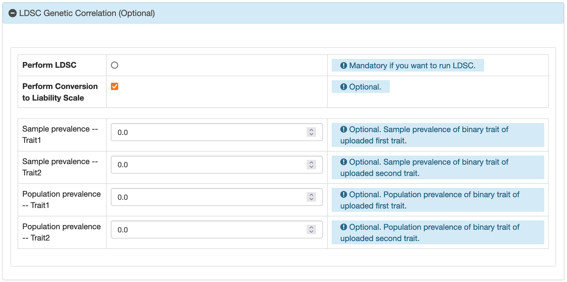

In pairwise analysis, BIGA provides a customized option for liability scale analysis of binary traits (traits that have two distinct values, e.g. presence or absence of a disease). When you enable the option "Perform Conversion to Liability Scale," you need to provide two pieces of information for each trait: the sample prevalence and the population prevalence. If a trait is not binary, you set its prevalence to 0, which is represented in the system as `nan` (not a number). If it is a binary trait, then the prevalence values should be between 0 and 1 (exclusive).

Default Script:
The provided script automates the process of genetic correlation analysis between two traits using LDSC:


if [ $samp_prev == "None" ]; then
 python2 $ldsc_path/ldsc.py   --rg $summary_statistics1,$summary_statistics2   --ref-ld-chr $ref_chr         --w-ld-chr $w_chr         --out $out
else
 python2 $ldsc_path/ldsc.py   --rg $summary_statistics1,$summary_statistics2   --ref-ld-chr $ref_chr         --w-ld-chr $w_chr         --out $out  --samp-prev $samp_prev --pop-prev $pop_prev
fi

Here, $summary_statistics1 and $summary_statistics2 represent the file paths for the first and second traits, respectively. When you opt for conversion to the Liability scale, additional flags --samp-prev and --pop-prev are included in the command to incorporate the prevalence parameters.

3. SumHer

Parameter settings: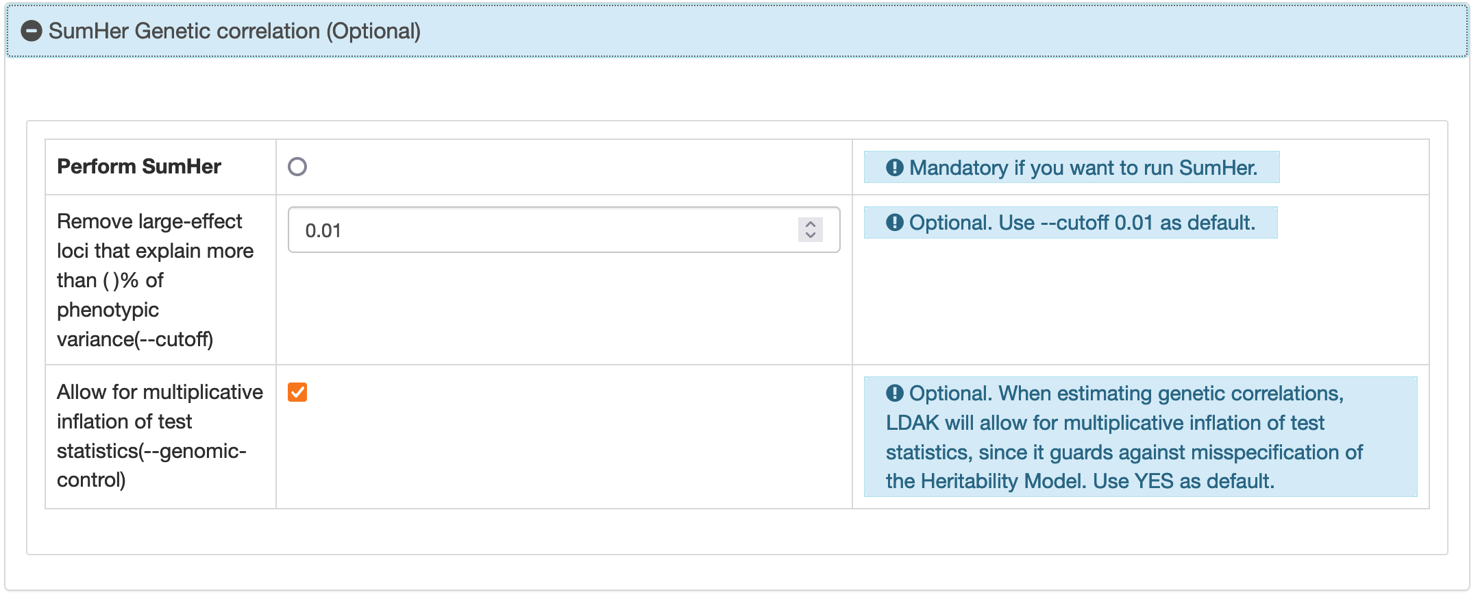

In this section, BIGA offers two specialized options: a cutoff parameter and the option to enable multiplicative inflation of test statistics. The cutoff parameter allows users to exclude loci with large effects that account for a significant portion of the phenotypic variance, with the default setting at 1%. When estimating genetic correlations, LDAK will allow for multiplicative inflation of test statistics, since it guards against misspecification of the heritability model. By default, BIGA enables this feature, but users have the option to disable it if needed by unchecking the corresponding box.

Default Script:
The provided script automates the process of genetic correlation analysis between two traits using SumHer:

                         
$sumHer_path/ldak5.2.$envir --summary $summary_statistics1 --summary2 $summary_statistics2 --sum-cors $out  --tagfile $sumHer_path/ldak.thin.hapmap.$popu.tagging --check-sums NO --allow-ambiguous YES --cutoff $cutoff --genomic-control $geno_control

$summary_statistics1 represents the first input summary data, either uploaded or queried by the user. $summary_statistics2 represents the second input summary data. $popu is a variable indicating the population-specific GWAS dataset, which can be either 'gbr' for the European population or 'eas' for East Asian. A SumHer analysis is conducted using the ldak5.2.$envir command. $envir can either be .mac or .linux depending on the operating system. The parameter $cutoff is employed to determine the threshold percentage for excluding loci with significant effects. Finally, the option --genomic-control is set to either YES or NO to decide on the allowance for multiplicative inflation in the test statistics.

4. LAVA

Parameter settings: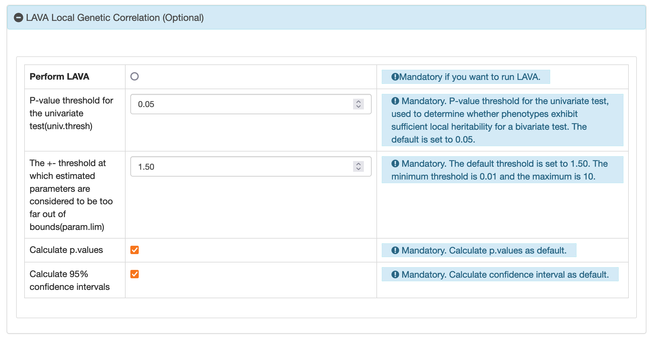

In this section, BIGA offers the following customized options: P-value threshold for the univariate test, the +- threshold at which estimated parameters are considered to be too far out of bounds, calculate p.values and calculate confidence intervals. The default p-value threshold is set to 0.05. The threshold for estimated parameters is set to 1.5. And BIGA calculates p.values and confidence intervals as default. All these parameters will be used in the function of

run.univ.bivar(locus, univ.thresh=uinv_thresh,
            p.values=p_values, CIs=ci, param.lim=parlim)

Default Script:


Rscript $lava_path/shell/2traits.R $lava_path $summary_statistics1 $summary_statistics2 $job_id $t1_name $t2_name $univ_thresh $p_values $ci $parlim  --no-restore --no-save

This is an example script of LAVA pairwise analysis, which is the command used to run R scripts from the command line.$summary_statistics1 represents the first input summary data, either uploaded or queried by the user. $summary_statistics2 represents the second input summary data. job_id is your job running id. t1_name,t2_name are the traits' names. univ_thresh is the p-value threshold for the univariate test. If ci is set to 'YES', then calculate confidence intervals. If p_values is set to `YES`, then calculate p-values. parlim is the +- threshold for estimated parameters.

5. Popcorn

Parameter settings: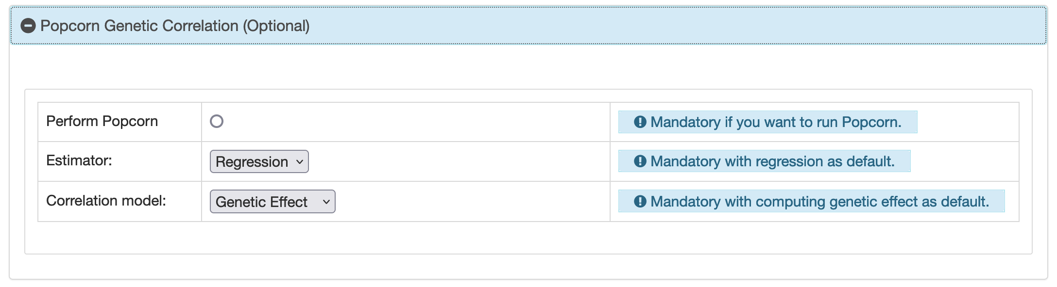

BIGA uses pre-calculated cross-population scores provided by Popcorn (https://www.dropbox.com/sh/37n7drt7q4sjrzn/AAAa1HFeeRAE5M3YWG9Ac2Bta). The score is for EUR and EAS 1000 genomes populations. When computing heritability and trans-ethnic genetic correlation of two set of summary statistics data, BIGA uses the function of Fit mode in Popcorn. The default estimator is regression, following Popcorn's recommendation due to the relative instability of the MLE method. You can select between Regression and MLE for the estimator. Another consideration in Popcorn is whether to compute the genetic effect correlation or the genetic impact correlation. BIGA uses --gen_effect as default since Popcorn believes that it's a more realistic model. BIGA uses MAF threshold of 0.05 by default since the larger the cutoff, the closer the genetic effect and the genetic impact results will be.

Default Script:


if [ $use_mle == "use_mle" -a $use_gen_effect == "use_gen_effect" ]; then
    out=$popcorn_path/2traits/log/$job_id/mle_gen_effect
    python -m popcorn fit -v 1  --use_mle --cfile $popcorn_path/ref/EUR_EAS_all_gen_imp.cscore --gen_effect --sfile1 $summary_statistics1 --sfile2 $summary_statistics2 $out
elif [ $use_mle == "use_mle" -a $use_gen_effect == "use_gen_impact" ]; then
    out=$popcorn_path/2traits/log/$job_id/mle_gen_imp
    python -m popcorn fit -v 1  --use_mle --cfile $popcorn_path/ref/EUR_EAS_all_gen_imp.cscore --sfile1 $summary_statistics1 --sfile2 $summary_statistics2 $out
elif [ $use_mle == "use_regression" -a $use_gen_effect == "use_gen_effect" ]; then
    out=$popcorn_path/2traits/log/$job_id/mle_reg_effect
    python -m popcorn fit -v 1 --cfile $popcorn_path/ref/EUR_EAS_all_gen_imp.cscore --gen_effect --sfile1 $summary_statistics1 --sfile2 $summary_statistics2 $out
else
    out=$popcorn_path/2traits/log/$job_id/mle_reg_imp
    python -m popcorn fit -v 1 --cfile $popcorn_path/ref/EUR_EAS_all_gen_imp.cscore --sfile1 $summary_statistics1 --sfile2  $summary_statistics2 $out
fi

$summary_statistics1 represents the first input summary data, either uploaded or queried by the user. $summary_statistics2 represents the second input summary data. EUR_EAS_all_gen_imp.cscore is the pre-calculated score. The script executes a series of conditional operations based on user-defined parameters (use_mle, use_gen_effect). The `if`, `elif`, and `else` statements direct the flow of execution.

4. Analysis Results and Log Files

4.1 Analysis Results

In the massive analysis result page, upon completion of your job, you have the option to download all the results. This can be done by clicking the "download" link, labeled as "result$job_id.tar.gz". This download includes several components: the BIGA log file, a log file documenting the method's execution, and the output from the method you selected. To view the primary genetic correlation analysis results, simply click on the 'go to result' option. In cases where your job did not complete successfully, the "result$job_id.tar.gz" file is still available for download, allowing you to access the log file and identify the reason for the failure.

The pairwise analysis result page shows similar information. If your job is successfully completed, you can download the entire set of results by clicking the "download" link, marked as "result$job_id.tar.gz". This package also contains the BIGA log file, the method run log file, and the output of the method you used. In instances where your job fails, the log file is accessible for review to determine the cause of the failure.

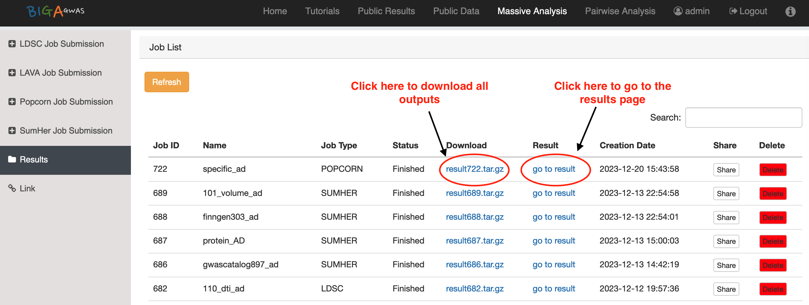
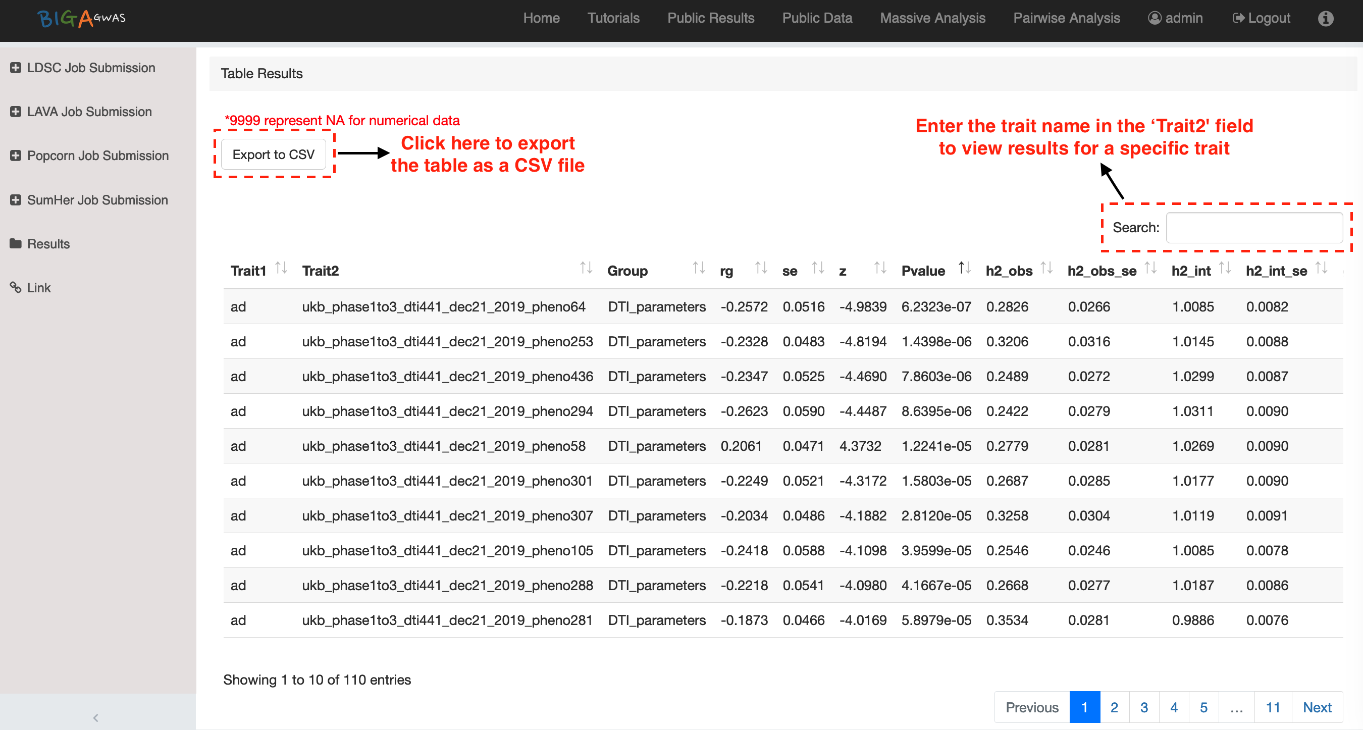
4.2 Read BIGA Log Files

The log file is structured in multiple sections, each providing specific information about the job being performed. Here is an example of querying ieu-b-30 from IEU OpenGWAS and then running Massive LDSC Analysis with PGC dataset.


************************************************************************
* BigaGWAS WorkShop
* version 1.1.0
* Yujue Li and Bingxin Zhao (2023-2024)
* Purdue University and University of Pennsylvania
* GNU General Public License v3
************************************************************************

This section is the masthead. It contains basic information about the software, including its name, version, authors, the associated institutions, and the license under which it is distributed.


==================================================================
****************** Running Massive LDSC Analysis *****************
Massive Analysis: Method=massive_ldsc Job_type=group_pgc Job_id=758.
Task running ID: 3c5c7887-c6fa-47e4-ae62-2d059051116b.
Current Job Settings:{'title': 'white blood cell count_649', 'username': 'admin', 'trait1_name': 'white blood cell count', 'job_id': '758', 'email_to': 'li4476@purdue.edu', 'need_harmonize': True, 'dropna': True, 'header': None, 'snp': False, 'query_error': False, 'chunksize_map_rsid': 500000, 'chunksize_harmo': 200000, 'gwas_catalog_chunksize': 10000, 'chunksize': 100000, 'convert_back_to_hg19': True, 'data_dir': '/Users/yujue/Documents/githubPackage/ldsc/data/758', 'log_dir': '/Users/yujue/Documents/githubPackage/ldsc/log/758', 'summary1_path': '/Users/yujue/Documents/githubPackage/ldsc/data/758/758_ldsc.sumstats.gz', 'job_type': 'massive_ldsc', 'choose_type': 'group_pgc', 'value': 'pgc', 'LDSC_PATH': '/Users/yujue/Documents/githubPackage/ldsc', 'population': 'european', 'group': 'PGC', 'chr': None, 'position': None, 'rsid': None, 'n': '', 'a1': None, 'a2': None, 'beta': None, 'eaf': None, 'pvalue': None, 'se': None, 'odds_ratio': None, 'zscore': None, 'hg_version': 'hg19', 'hg19_final_data': '/Users/yujue/Documents/githubPackage/ldsc/data/758/758.txt', 'link1': 'https://gwas.mrcieu.ac.uk/files', 'sample_size_catalog': '563946', 'query_party': 'opengwas', 'select_trait1': 'querying', 'query_id': 'ieu-b-30', 'celery_id': '3c5c7887-c6fa-47e4-ae62-2d059051116b'}.

In this section, the log file provides an overview of the current analysis being run. It includes the method used (`massive_ldsc`), the type of job (`group_pgc`), and a unique job ID (`758`). There's also a task running ID, which is likely a unique identifier for this specific instance of the task.


************************* Querying from openGWAS ***********************
Task running script:...
Read VCF File.
Finish reading VCF file.
Starting to convert into harmonize format.
Querying Finished. Time consuming: 12495.486000299454 seconds.

This part details the querying process from IEU OpenGWAS, including script execution and file processing. It provides information on reading the downloaded VCF files and the time taken to complete these processes. Here, it is focused on converting data into the format for harmonization.


*********** Starting to map rsid to chromosome and position ************
Mapping dbSNP156_GRCh38_chr_12-3.txt : 443.08141112327576 seconds
Mapping dbSNP156_GRCh38_chr_10-3.txt : 480.74914479255676 seconds
Mapping dbSNP156_GRCh38_chr_14-1.txt : 582.9732220172882 seconds
...
*********************** Starting to harmonize data **********************
*********** Starting to infer the direction of the strand ***************
Infering the orientation of palindromatic variants by randomly selecting 5% of varints.

Chromosome 7: Counter({'Forward strand variant': 63390, 'Palindormic variant': 10876, 'Reverse strand variant': 181})
Chromosome 8: Counter({'Forward strand variant': 61659, 'Palindormic variant': 11539, 'Reverse strand variant': 24})
Chromosome 6: Counter({'Forward strand variant': 69403, 'Palindormic variant': 11477, 'Reverse strand variant': 182, 'Invalid variant for harmonization': 1})
Chromosome 5: Counter({'Forward strand variant': 71753, 'Palindormic variant': 12207})
...
Overall Forward strand rate: 0.998454, Reverse strand rate:0.001546.

Harmonizing summary statistics data.
Chromosome 7, Strand Inference Summary:
Counter({'Forward strand variant': 1268728, 'Palindormic variant': 218235, 'Reverse strand variant': 3702, 'Invalid variant for harmonization': 4})
Chromosome 7, Harmonization summary:
Counter({'Forward strand; Correct orientation; Already harmonised': 1267544, 'Palindromic; Assume forward strand; Correct orientation; Already harmonised': 217334, 'Reverse strand; Correct orientation; Already harmonised': 3462, 'Forward strand; Flipped orientation; Requires harmonisation': 1184, 'Palindromic; Assume forward strand; Flipped orientation; Requires harmonisation': 901, 'Reverse strand; Flipped orientation; Requires harmonisation': 240})
...
Harmonization ends. Time consuming: 6123.922087430954 seconds.

This section covers the mapping of rsid to chromosome and position aligned with GRCh38 and the time taken for each chromosome. It then goes into harmonizing the summary statistics data, inferring the direction of the strand, providing detailed summaries and counts for each chromosome. The section ends by noting the total time spent on harmonization.


*************** Combining and Sorting Harmonized data ****************
Combining and Sorting ends. Time consuming: 173.49580812454224 seconds.

This section indicates that the harmonized data has been combined and sorted by chromosomes. The time taken for this process is noted, allowing for performance tracking.


************ Starting to convert back to GRCh37 version ****************
1366 positions did not align with the GRCh37 reference.

Liftover to GRCh37 Finished. Time Consuming: 454.24938797950745 seconds.

Here, the log file records the process of converting the data back to the GRCh37 for analysis because LDSC needs position built on GRCh37 version. It specifically notes that 1366 positions did not align with the GRCh37 reference file. The duration of this liftover process is also recorded.


********* Converting into sumstats.gz for use in LDSC analysis *********
Converting Finished. Time Consuming: 129.55129599571228 seconds.

This part of the log indicates the final conversion of the data into `sumstats.gz` format, which is used in LDSC analysis. The time taken for this conversion is provided.


************************* Running LDSC Software ************************
Starting to run 24 PGC psychiatric disorders and other diseases traits.
Command line:
sh /Users/yujue/Documents/githubPackage/bigagwas/static/shell/pgc_24.sh 758 ...

This section shows the initiation of the LDSC software to analyze 24 PGC psychiatric disorders and other brain diseases traits. It includes the command line used to run the analysis.


*********************************************************************
* LD Score Regression (LDSC)
* version 1.1.0
* (C) 2014-2019 Brendan Bulik-Sullivan and Hilary Finucane
* Broad Institute of MIT and Harvard / MIT Department of Mathematics
* GNU General Public License v3
*********************************************************************
Call:
./ldsc.py \
--ref-ld-chr /Users/yujue/Documents/githubPackage/ldsc/eur_w_ld_chr/ \
--out /Users/yujue/Documents/githubPackage/ldsc/log/758/phenoone \
--rg /Users/yujue/Documents/githubPackage/ldsc/data/758/758_ldsc.sumstats.gz,/Volumes/sandisk/summary_statistics/harmo/ldsc/data/pgc/hg19/8_ocd_aug2017.sumstats.gz
...

Finally, the log file gives the output of the LDSC software being used. More information about this section is provided by LDSC software itself.

5. Queue System and Periodic Jobs

5.1 Queue System

There are two queue systems implemented by Celery to manage different types of analyses based on their memory requirements. The first queue runs Massive LDSC Analysis, Massive SumHer Analysis, Pairwise LDSC Analysis and Pairwise SumHer Analysis. This queue is designed to be memory-efficient, allowing up to three tasks to run concurrently since LDSC and SumHer have lower memory demands. The second queue runs Massive LAVA Analysis, Massive POPCORN Analysis, Pairwise LAVA Analysis and Pairwise POPCORN Analysis. Unlike the first queue, this one is more memory-intensive and is structured to handle only one task at a time. These two queue systems create a more stable and effective environment for running various genomic analyses.

5.2 Periodic Jobs

BIGA incorporates two key periodic jobs to maintain its data and operations.

Daily GWAS Catalog Update

This function is scheduled every day at 5:30 AM Eastern Time to keep the GWAS Catalog available list up-to-date. The GWAS Catalog offers a daily updated harmonized data list (http://ftp.ebi.ac.uk/pub/databases/gwas/summary_statistics), and in order to maintain synchronization with the GWAS Catalog, BIGA will also refresh its list on a daily basis.

Daily Input Files Cleanup

This function is scheduled every day at 5:30 AM Eastern Time to clean out input files stored in BIGA for more than 7 days. Considering that the summary statistics data typically exceeds 500 MB, this process is crucial for maintaining efficient data usage, especially with numerous jobs in progress. BIGA temporarily saves your input files for 7 days, after which all input files are deleted based on the last update date of your job. This regular cleanup routine can keep the system running smoothly and ensure the data storage is effectively managed for both current and future users.

6. Other Functions

6.1 Email Notification

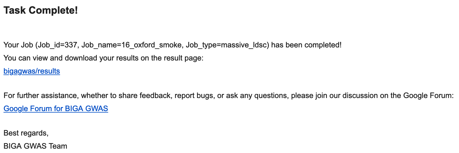
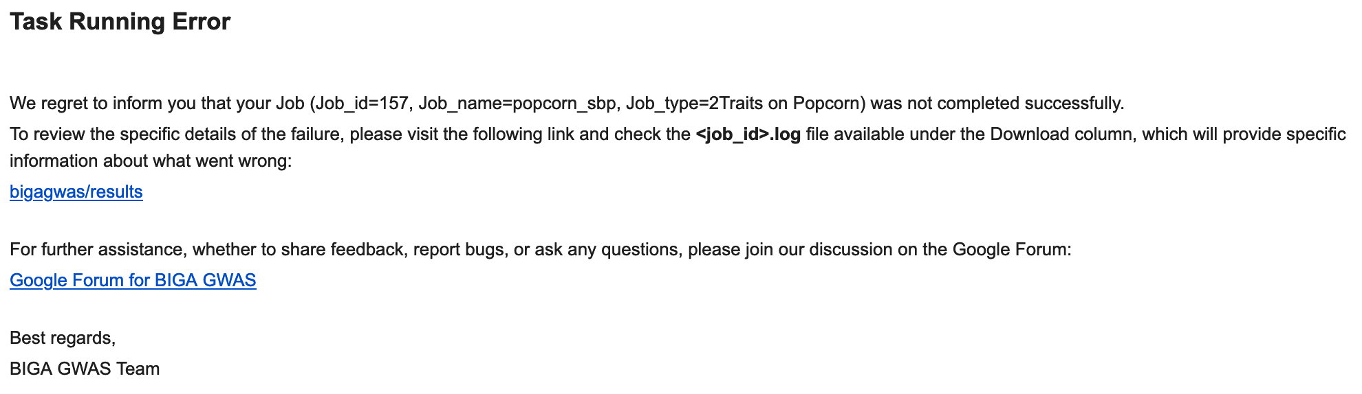
After a job has completed, regardless of whether it ended successfully or encountered a error, you will be notified via email. You will receive a Task Complete email notification if the job completes successfully. The following is an example.

You will receive a Task Running Error email if the job fails. The following is an example.

Please ensure to check your junk or spam email folder as well, in case any notifications were mistakenly directed there.

6.2 Public Data

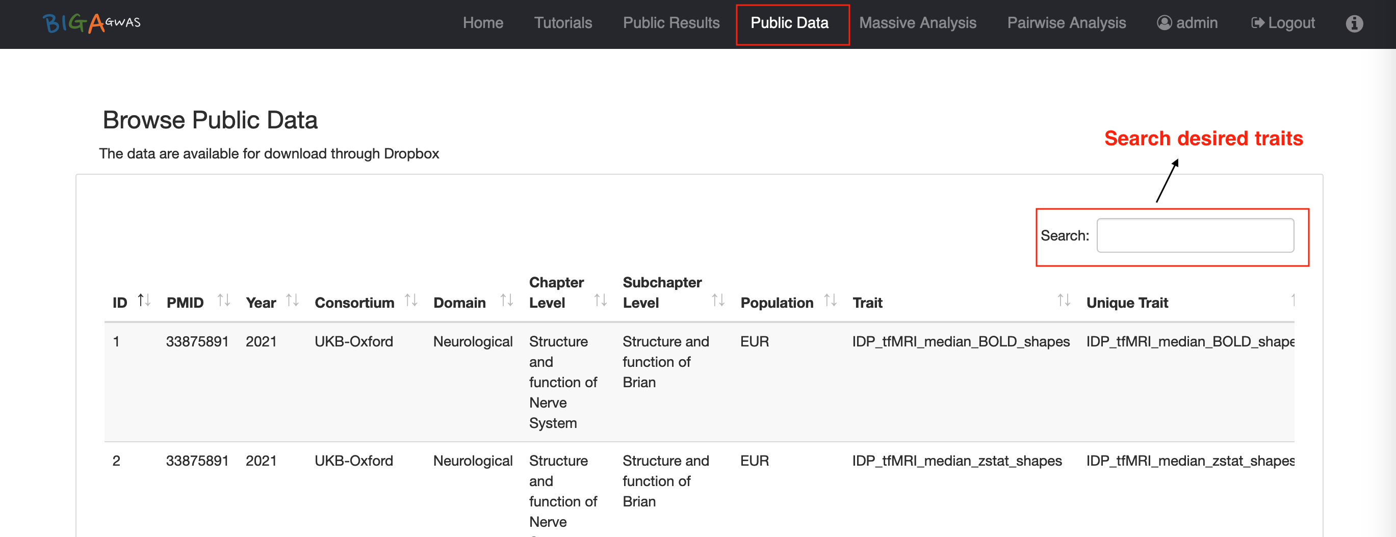
BIGA now provides UKB Oxford dataset, which can be downloaded through our cloud data storage platform.

6.3 Public Results

If you find any result particularly useful, you have the option to share it publicly, allowing other users to view and download it.

7. Description Examples

Here we present sample descriptions for using each method through the BIGA platform. Users may incorporate similar language into the methods section of their papers or reports. It is important to properly cite the original papers related to both the methods and datasets being used in the analysis.

7.1 Method: LDSC

We performed genetic correlation analysis using LDSC (https://github.com/bulik/ldsc, version 1.0.1) via the BIGA platform (version 1.1.2, http://bigagwas.org/). The LD scores were from the 1000 Genomes data and were provided by LDSC. This analysis was focused on HapMap3 variants and the variants in the major histocompatibility complex region were removed. Before performing the LDSC analysis, the GWAS summary statistics were harmonized by BIGA, following the harmonization pipeline of GWAS Catalog (https://www.ebi.ac.uk/gwas/docs/methods/summary-statistics). We screened all curated GWAS summary statistics of European ancestry provided by BIGA, including UK Biobank (UKB) traits from Neale lab, brain and body imaging traits from UKB Oxford and BIG-KP, UKB plasma proteomic data, FinnGen, Psychiatric Genomics Consortium and other brain disorders, and GWAS Catalog. We used default values for other parameters and more details can be found at http://bigagwas.org/documentation.

7.2 Method: SumHer

We performed genetic correlation analysis using SumHer (http://dougspeed.com/genetic-correlations/, version ldak5.2) via the BIGA platform (version 1.1.2, http://bigagwas.org/). The tagging files are pre-computed based on reference SNPs, which were the 10M SNPs that were both present in the 1000 Genomes Project and had MAF>0.005. We removed variants that explained more than 1% of phenotypic variance. Before performing the SumHer analysis, the GWAS summary statistics were harmonized by BIGA, following the harmonization pipeline of GWAS Catalog (https://www.ebi.ac.uk/gwas/docs/methods/summary-statistics). We screened all curated GWAS summary statistics of European ancestry provided by BIGA, including UK Biobank (UKB) traits from Neale lab, brain and body imaging traits from UKB Oxford and BIG-KP, UKB plasma proteomic data, FinnGen, Psychiatric Genomics Consortium and other brain disorders, and GWAS Catalog. The P-value for estimated genetic correlation is calculated by BIGA using the Wald test. We used default values for other parameters and more details can be found at http://bigagwas.org/documentation.

7.3 Method: LAVA

We performed local genetic correlation analysis using LAVA (https://github.com/josefin-werme/LAVA/, version 0.1.0) via the BIGA platform (version 1.1.2, http://bigagwas.org/). Reference genotype data was created from Phase 3 of the 1,000 Genomes Project and was downloaded from CTG Lab (https://ctg.cncr.nl/software/magma, section “Reference data”). Before performing the LAVA analysis, the GWAS summary statistics were harmonized by BIGA, following the harmonization pipeline of GWAS Catalog (https://www.ebi.ac.uk/gwas/docs/methods/summary-statistics). We screened all curated GWAS summary statistics of European ancestry provided by BIGA, including UK Biobank (UKB) traits from Neale lab, brain and body imaging traits from UKB Oxford and BIG-KP, UKB plasma proteomic data, FinnGen, Psychiatric Genomics Consortium and other brain disorders, and GWAS Catalog. We used default values for other parameters and more details can be found at http://bigagwas.org/documentation.

7.4 Method: Popcorn

We performed cross-population genetic correlation analysis using Popcorn (https://github.com/brielin/Popcorn, version 1.0.0) via the BIGA platform (version 1.1.2, http://bigagwas.org/). The cross-population scores were computed from the 1000 Genomes data and downloaded from Popcorn. Before performing the Popcorn analysis, the GWAS summary statistics were harmonized by BIGA, following the harmonization pipeline of GWAS Catalog (https://www.ebi.ac.uk/gwas/docs/methods/summary-statistics). We screened all curated GWAS summary statistics of East Asian ancestry provided by BIGA, including Biobank Japan and CHIMGEN. We used the regression estimator and genetic effect model as recommended by Popcorn. The p-value for the hypothesis, which assume that the correlation is 0, is calculated using the Wald test by BIGA. We used default values for other parameters and more details can be found at http://bigagwas.org/documentation.

Documentation of BIGA GWAS

Table of Contents

1. Data Processing

2. Curated Datasets

3. Analysis

4. Analysis Results and Log Files

5. Queue System and Periodic Jobs

6. Other Functions

7. Description examples

1. Data Processing

1.1 Data Processing Diagram

1.2 Table 1. Required columns for harmonization and BIGA analysis

1.3 Build Input Files

Header Detection Rules

Missing value

Parameters

Notes

GWAS Catalog Data

IEU OpenGWAS Data

Neale Lab Data

1.4 Data Harmonization Pipeline

1.5 Harmonization Codes

1.6 Query Data from GWAS Catalog

Step 1: Searching for the Trait

Step 2: Verifying Data Availability

Step 3: Confirming the trait is query-able by BIGA

1.7 Query Data from IEU OpenGWAS

Step 1: Searching for the Trait

Step 2: Confirming the trait is query-able by BIGA

1.8 Query Data from Neale Lab

2. Curated Dataset

2.1 Brain and Organ Imaging Traits

Description

Reference

Data Processing

2.2 UK Biobank (Neale Lab)

Description

Reference

Data Processing

2.3 UKB Oxford Brain Imaging Traits

Description

Reference

Data Processing

2.4 Biobank Japan

Description

Reference

Data Processing

2.5 UKB-PPP European Protein GWAS

Description

Reference

Data Processing

2.6 FinnGen

Description

Reference

Data Processing

2.7 PGC (Psychiatric Genomics Consortium) and Other Brain Disorders

Description

Reference

Data Processing

2.8 GWAS Catalog

Description

Reference

Data Processing

2.9 CHIMGEN

Description

Reference

Data Processing

3. Analysis Methods

3.1 Massive LDSC Analysis

Reference

Curated Dataset

Input File Build

Configuration Settings

Default Script

3.2 Massive SumHer Analysis

Reference

Curated Dataset

Input File Build

Configuration Settings

Default Script